Electro-Hydraulic Active Suspension for Rollover Prevention: Control Performance and Actuator Design Requirements

Jeongwoo Lee

doi:10.22680/kasa2026.18.3.061

Preview

Journal of Auto-vehicle Safety Association. 30 September 2026. 61-77
https://doi.org/10.22680/kasa2026.18.3.061

Electro-Hydraulic Active Suspension for Rollover Prevention: Control Performance and Actuator Design Requirements

Jeongwoo Lee¹^†

¹Assistant Professor, School of Automotive Engineering, Kyungpook National University

^{†Corresponding Author}

ABSTRACT

This study proposes an active body control system model that supplies the required hydraulic pressure only during active roll control to reduce the high energy consumption associated with conventional active suspension systems. To this end, a commercially available electro-hydraulic actuator was modeled, and a control algorithm was constructed by combining roll-angle estimation and rollover index calculations. Co-simulation results using CarSim and Simulink demonstrated that the vehicle equipped with the proposed active suspension system reduced the rollover index by more than 70% compared with the passive suspension system and maintained the roll angle within 5 degrees under emergency driving conditions, confirming its rollover prevention capability. Furthermore, the actuator requirement analysis showed that the maximum simulated cylinder pressure was 82.5 bar under the 0.5 g condition. This value was rounded upward to define a peak operating-pressure requirement of 85 bar, corresponding to a required operating load of approximately 664.6 kgf when a conservative nominal piston area of 7.9 cm² was used. A design pressure rating of at least 100 bar was recommended, providing a 17.6% pressure margin above the 85-bar operating requirement. These results provide design guidelines for the motor, actuator, and overall system configuration of future electro-hydraulic active suspension systems.

Keywords

Vehicle suspension

Slow active suspension

Hydraulic system

Rollover Index

Roll control

MAIN

1. Introduction
2. Active suspension system
2.1. Active Suspension System Modeling
2.2. Active Suspension Actuator Performance Rig Test
3. Vehicle dynamics control for active roll control
3.1. Vehicle roll angle estimation
3.2. Rollover Index
4. Simulation Results
4.1. Rollover Simulation
4.2. Dynamic Maneuver Simulation
5. Conclusion and Future Work

1. Introduction

As safety and ride comfort in automobiles have become increasingly important, vehicle suspension systems have evolved in various ways. With recent technological advancements, active suspension systems equipped with active actuators that transmit force to the sprung body have been actively researched. In particular, systems in which the spring and piston are configured in series to control the vehicle’s behavioral state by displacing the spring have been researched, developed, and commercialized (1)-(3). The in-series suspension can provide performance comparable to a fully active suspension with lower actuation demand. However, conventional implementations commonly use a hydraulic power unit that maintains a nominal supply pressure of approximately 200 bar, so pressure-maintenance and throttling losses may remain even when the full actuator output is not required.

The present system instead commands the motor-driven pressure source to generate hydraulic pressure only when active roll control is requested. Because total electrical energy consumption also depends on pump efficiency, leakage, valve losses, and the driving duty cycle, a complete energy-saving percentage cannot be inferred from supply pressure alone. Accordingly, the energy-saving potential is evaluated in Section 4.2 using a first-order hydraulic pressure-power comparison based on the simulated actuator pressure and flow demand.

In this study, we analyze the parameters to be considered for determining system performance and specifications by simulating a serial active suspension actuator model using the analysis and test results of existing commercialized hardware systems.

Section 2 presents the system modeling and performance test analysis of a mass-produced electro-hydraulic strut module. Section 3 describes the roll-angle estimation method, rollover index, and active roll-control algorithm used to evaluate rollover prevention performance. Section 4 presents the simulation results of the developed model, and Section 5 concludes the paper.

2. Active suspension system

2.1. Active Suspension System Modeling

2.1.1 Quarter-Car Dynamics

The quarter-car model equipped with an electro-hydraulic actuator arranged in series with the suspension spring is shown in Fig. 1. Fluid inflow into or out of the actuator changes the actuator displacement and, consequently, the deformation and transmitted force of the suspension spring. The corresponding equations of motion are given by Eqs. (1)-(3).

https://cdn.apub.kr/journalsite/sites/kasa/2026-018-03/N0380180306/images/kasa_18_03_06_F1.jpg

Fig. 1

Active suspension quarter-car model

(1)

m_{s} \ddot{x_{s}} = - k_{s} (x_{s} - x_{u}) + k_{s} (x_{s} - x_{a}) - F_{c}

(2)

F_{a} = k_{s} (x_{s} - x_{a}) = A_{a} p_{a}

(3)

m_{u} \ddot{x_{u}} = k_{s} (x_{s} - x_{u}) - k_{s} (x_{s} - x_{a}) + F_{c} - F_{t i r e}

In Eqs. (1)-(3), $m_{s}$ and $m_{u}$ are the sprung and unsprung masses, respectively [kg], while $x_{s}$ , $x_{u}$ , and $x_{a}$ are the vertical displacements of the sprung mass, unsprung mass, and actuator piston, respectively [m]. The symbols $m_{u}$ and $x_{u}$ correspond to $m_{w}$ and $x_{w}$ in Fig. 1. The parameter $k_{s}$ denotes the suspension spring stiffness [N/m], $F_{c}$ is the suspension damping force [N], and $F_{t i r e}$ is the vertical tire force [N]. The spring force is expressed as $F_{s} = k_{s} (x_{s} - x_{a})$ , and the series arrangement gives $F_{a} = F_{s} = A_{a} p_{a}$ , where $F_{a}$ is the actuator force [N], $A_{a}$ is the effective hydraulic piston area [m²], and $p_{a}$ is the actuator cylinder pressure [Pa]. When the actuator model in Eqs. (4)-(8) is coupled to the quarter-car model, $x_{a} = x_{r}$ , $A_{a} = A$ , and $p_{a} = p_{c}$ are used. Overdots denote derivatives with respect to time, and the positive directions of the displacement variables are defined in Fig. 1.

2.1.2 Hydraulic Actuator

A detailed schematic view considering the hydraulic circuit of the piston part is shown in Fig. 2.

https://cdn.apub.kr/journalsite/sites/kasa/2026-018-03/N0380180306/images/kasa_18_03_06_F2.jpg

Fig. 2

Schematic of the hydraulic actuator and valve

The valve is connected to an input terminal via an electric motor pump and a reservoir that provides constant high pressure, and to the output terminal via the pistons of each wheel. Flow rate control is possible based on the input voltage value. Since a stroke sensor is installed inside the cylinder, the desired piston stroke can be controlled according to the vehicle's movement state.

2.1.3 Actuator Dynamics

Fig. 3 illustrates the steps for generating pressure in the actuator. First, the valve was modeled by separating its electrical and hydraulic characteristics. Receiving voltage as input, the valve outputs a flow rate based on the position of the valve piston. When hydraulic pressure passes through the tube and reaches the cylinder, the inflow flow rate is determined by the pressure difference between the input end and the inside of the cylinder, which in turn determines the position of the cylinder piston. If this entire process is diagrammed as a state space model, it can be modeled as shown in Eq. (4) and (5).^(4~⁶⁾

https://cdn.apub.kr/journalsite/sites/kasa/2026-018-03/N0380180306/images/kasa_18_03_06_F3.jpg

Fig. 3

Block diagram of the hydraulic actuator

(4)

x_{h} = {[\begin{matrix} x_{h, 1} & x_{h, 2} & x_{h, 3} & x_{h, 4} & x_{h, 5} & x_{h, 6} & x_{h, 7} \end{matrix}]}^{T} = [\begin{matrix} x_{r} & \dot{x_{r}} & p_{c} & p_{v} & q_{c} & x_{v} & \dot{x_{v}} \end{matrix}]

(5)

[\begin{matrix} {\dot{x}}_{h, 1} \\ {\dot{x}}_{h, 2} \\ {\dot{x}}_{h, 3} \\ {\dot{x}}_{h, 4} \\ {\dot{x}}_{h, 5} \\ {\dot{x}}_{h, 6} \\ {\dot{x}}_{h, 7} \end{matrix}] = [\begin{matrix} x_{h, 2} \\ \frac{1}{m_{r}} [A \cdot x_{h, 3} - F_{L} (x_{h, 1}) - d_{r} x_{h, 2} + m_{r} g] \\ \frac{β}{V_{0} + A x_{h, 1}} [x_{h, 5} - A \cdot x_{h, 2}] \\ \frac{1}{C_{h}} [s g n^{+} (x_{h, 6}) k_{s v} \sqrt[]{|p_{v} - x_{h, 4}|} - s g n^{+} (- x_{h, 6}) k_{s v} \sqrt[]{|x_{h, 4} - p_{T}|}] \\ \frac{1}{L_{h}} [x_{h, 4} - x_{h, 3}] \\ x_{h, 7} \\ - \frac{2 d_{v}}{T_{v}} x_{h, 7} - \frac{1}{T_{v}^{2}} x_{h, 6} \end{matrix}] + [\begin{matrix} 0 \\ 0 \\ 0 \\ 0 \\ 0 \\ 0 \\ \frac{k_{v}}{T_{v}^{2}} \end{matrix}] u

The hydraulic actuator is represented by the seven-state vector in Eq. (4), where $x_{r}$ [m] and $\dot{x_{r}}$ [m/s] are the actuator-rod displacement and velocity, $p_{c}$ [Pa] and $p_{v}$ [Pa] are the cylinder and valve-line pressures, $q_{c}$ [m³/s] is the flow rate into the cylinder, and $x_{v}$ [m] and $\dot{x_{v}}$ [m/s] are the valve-spool displacement and velocity, respectively.

In Eq. (5), $m_{r}$ is the equivalent moving mass of the piston [kg], $A$ is the effective piston area [m²], $F_{L}$ ( $x_{r}$ ) is the mechanical load force acting on the piston [N], and $d_{r}$ is the viscous friction coefficient [N·s/m]. The quantities $β$ , $V_{0}$ , $C_{h}$ , and $L_{h}$ denote the effective bulk modulus of the hydraulic fluid [Pa], initial cylinder volume [m³], hydraulic capacitance [m³/Pa], and hydraulic inertance [Pa·s²/m³], respectively. The supply and tank pressures are denoted by $p_{v}$ and $p_{T}$ [Pa], while $k_{s v}$ is the valve flow coefficient [m²/(s·√Pa)]. The parameters $K_{v}$ , $T_{v}$ , and $d_{v}$ represent the valve displacement gain [m/V], valve time constant [s], and dimensionless valve damping ratio, respectively, and $g$ denotes gravitational acceleration [m/s²].

The control input $u (t) = u_{v, h y} (t)$ is the valve command voltage [V]. The valve input and the corresponding flow relation are defined by Eqs. (6)-(8).

(6)

u (t) = u_{v, h y}

(7)

s g n^{+} (x_{i}) = \{\begin{cases} x_{i} f o r x_{i} > 0 \\ 0 e l s e \end{cases}

(8)

q_{v} = s g n^{+} (x_{h, 6}) k_{s v} \sqrt{|p_{v} - x_{h, 4}|} - s g n^{+} (- x_{h, 6}) k_{s v} \sqrt{|x_{h, 4} - p_{T}|}

In Eq. (8), $q_{v}$ is the flow rate through the control valve [m³/s]. The positive-part operator sgn⁺(·), defined in Eq. (7), represents the supply-to-cylinder and cylinder-to-tank flow paths separately according to the valve-spool direction. Pressures are evaluated in pascals in the governing equations, although bar is used when reporting the numerical simulation and test results.

The hydraulic-model parameters adopted from Ref. (5) are summarized in Table 1. Each value is reported in SI units, with engineering-unit equivalents added for the principal geometric quantities. In particular, the piston area is $A$ = 4.7263 × 10^-4 m² (4.7263 cm²), the initial cylinder volume is $V_{0}$ = 4.3367 × 10^-8 m³ (0.043367 cm³), and the tube flow cross-sectional area is $A_{t}$ = 3.228 × 10^-5 m² (0.3228 cm²). These parameters determine the pressure-to-force conversion, cylinder pressure-volume dynamics, and tube-flow dynamics in Eq. (5), respectively.

Table 1.

Parameters of the reference hydraulic actuator model (Ref. 5)

Component	Parameter	Symbol	Value (SI and engineering units)
Hydraulic cylinder	Piston area	$A$	4.7263 × 10^-4 m² (4.7263 cm²)
	Initial cylinder volume	$V_{0}$	4.3367 × 10^-8 m³ (0.043367 cm³)
	Piston mass	$m_{r}$	9.8816 kg
	Friction coefficient	$d_{r}$	7.0006 × 10³ N·s/m
	Maximum stroke	${\hat{x}}_{r}$	0.0859 m (85.9 mm)
	Gravitational acceleration	g	9.81 m/s²
Tubes	Tube flow cross-sectional area	$A_{t}$	3.228 × 10^-5 m² (0.3228 cm²)
Tubes	Tube length	$l_{t}$	2.23 m

2.1.4 System Response Compensation Control

When the valve input voltage is positive, the flow path between the pump and the cylinder is connected. When the input voltage is negative, the flow path between the cylinder and the reservoir is connected. First, when the valve control input is positive (u≥0), the pressure difference can be calculated as in Eq. (9), and when the valve control input is negative (u>0), it can be calculated as in Eq. (10).

(9)

∆ p_{p o s} (p_{c}) = (p_{v} - p_{c}) - (p_{v} - p_{c, 0}) = p_{c, 0} - p_{c}

(10)

∆ p_{n e g} (p_{c} = p_{c, 0}) = p_{c, 0} - p_{0}

This result indicates that differences in internal pressure affect responsiveness. Therefore, compensation control is required to address this and reduce the responsiveness difference. The compensated input voltage is calculated separately for the valve control amount, depending on the control direction, and is given by Eq. (11).

(11)

u = \frac{u^{*}}{(\frac{∆ p}{p_{0}} + 1)} with ∆ p = \{\begin{cases} p_{c, 0} - p_{c}, if u \geq 0 \\ p_{c} - p_{0}, if u < 0 \end{cases}

In the above, u^* represents the compensated controller input value. The simulation result with the above compensation applied is shown in Fig. 4.

https://cdn.apub.kr/journalsite/sites/kasa/2026-018-03/N0380180306/images/kasa_18_03_06_F4.jpg

Fig. 4

Response performance of the actuator displacement

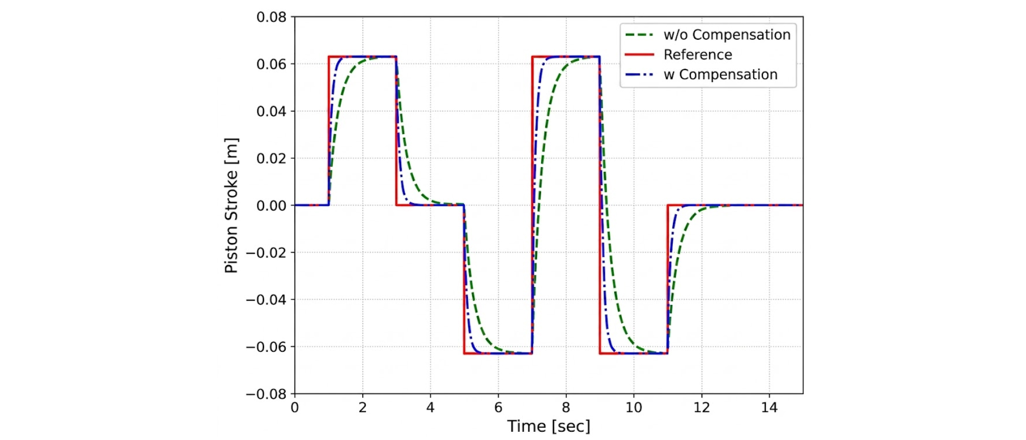
The analysis of the piston's responsiveness after internal system pressure compensation, relative to the target stroke, is shown in Table 2.

Table 2.

Response time of the actuator’s linear motion

Stroke [mm]	u ≥ 0 [ms]	u < 0 [ms]
0 ↔ 20	175	162
0 ↔ -20	177	165
0 ↔ 40	291	296
0 ↔ -40	292	308
0 ↔ 60	423	432
0 ↔ -60	424	454

The figures and table above show the experimental results for an initial load of 500 kgf (64 bar) in the CarSim S-Class. Across all stroke commands, the maximum difference in response time between the (u ≥ 0) and (u > 0) control directions was 30 ms, indicating that the pressure-difference compensation effectively reduced the directional variation in actuator response.

2.2. Active Suspension Actuator Performance Rig Test

2.2.1 Test Configuration

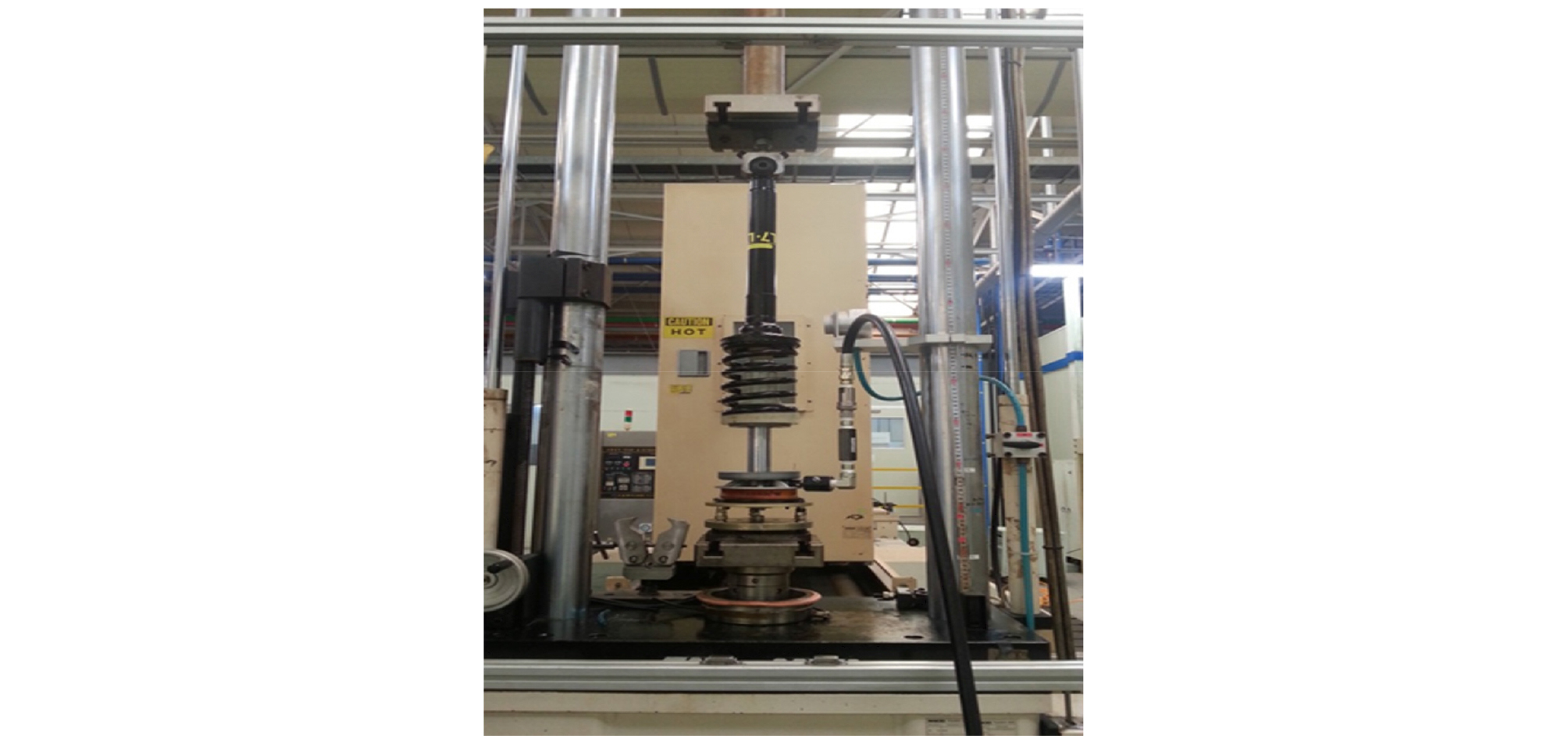
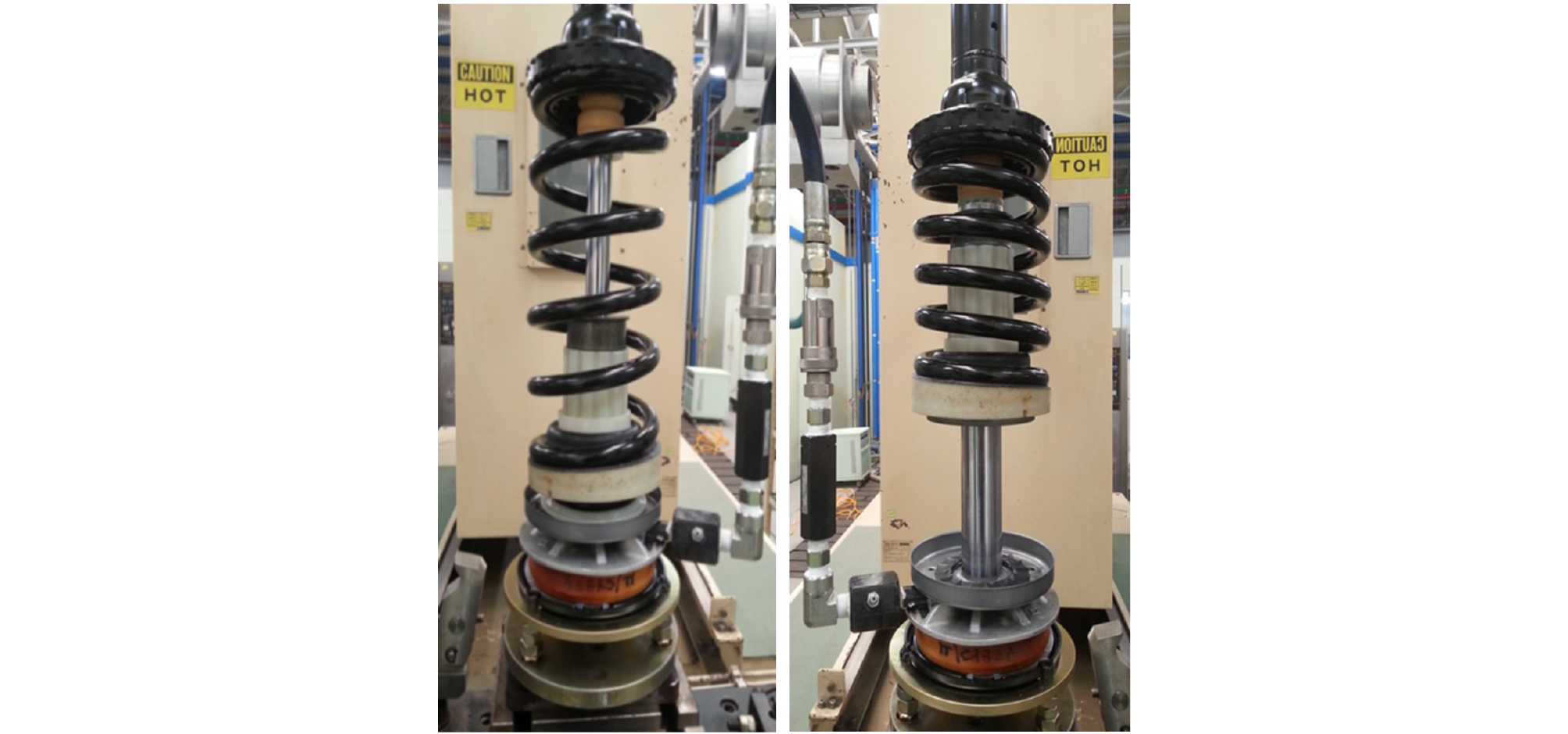
To identify the actuator parameters used in the simulation, a commercially available electro-hydraulic strut was vertically mounted on the test rig, as shown in Fig. 5. The actuator was connected to a load cell with a capacity of 3,000 kgf and to a hydraulic pump capable of supplying up to 200 bar. For the quasi-static pressure test, the cylinder pressure was increased from 0 to 110 bar in 10 bar increments. At each pressure step, the cylinder pressure, piston displacement, and transmitted load were recorded after the actuator response reached a steady value. The built-in stroke sensor was used to measure piston displacement, while the load cell was used to monitor the transmitted force. The actuator configurations at the minimum and maximum stroke positions are shown in Fig. 6. The measured pressure–displacement and pressure–load characteristics were used to determine the maximum stroke and effective hydraulic area, respectively, and the identified parameters were subsequently incorporated into the vehicle dynamics model.

https://cdn.apub.kr/journalsite/sites/kasa/2026-018-03/N0380180306/images/kasa_18_03_06_F5.jpg

Fig. 5

Active suspension actuator test setup

https://cdn.apub.kr/journalsite/sites/kasa/2026-018-03/N0380180306/images/kasa_18_03_06_F6.jpg

Fig. 6

Actuator minimum (left) & maximum (right) stroke

2.2.2 System Pressure Test Results

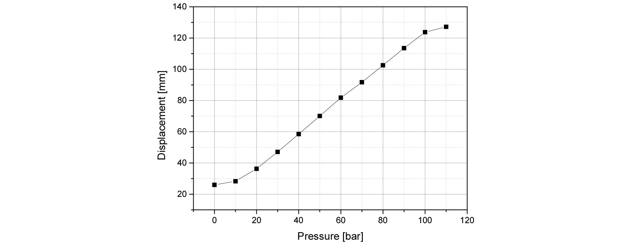
The actuator displacement results obtained from the rig test at different pressures are shown in Fig. 7. The displacement offset at 0 bar results from the small internal spring and does not affect the subsequent identification of the actuator parameters. The effective hydraulic piston area and maximum actuator stroke identified from the pressure-load and pressure-displacement data are listed in Table 3 in both SI and engineering units. The measured values are $A_{e}$ = 7.960 × 10^-4 m² (7.960 cm²) and $x_{r, m a x}$ = 0.1270 m (127.0 mm), respectively. These identified parameters were used for the actuator force-capacity and stroke-requirement analyses. Table 1 and Table 3 describe different hardware: Table 1 contains parameters adopted from the reference hydraulic actuator model, whereas Table 3 contains parameters identified from the commercial electro-hydraulic strut tested in this study.

https://cdn.apub.kr/journalsite/sites/kasa/2026-018-03/N0380180306/images/kasa_18_03_06_F7.jpg

Fig. 7

Actuator displacement according to hydraulic pressure

Table 3.

Experimentally identified parameters of the commercial actuator

Main design parameter	Value (SI and engineering units)
Effective hydraulic piston area, $A_{e}$	7.960 × 10^-4 m² (7.960 cm²)
Maximum actuator stroke, $x_{r, m a x}$	0.1270 m (127.0 mm)

3. Vehicle dynamics control for active roll control

3.1. Vehicle roll angle estimation

The lateral, roll, and longitudinal motion of a vehicle can be expressed by Eqs. (12)-(14).

(12)

{\dot{v}}_{y} = - ω_{z} v_{x} + ω_{x} v_{z} + a_{y} - g \sin ϕ \cos θ

(13)

\dot{ϕ} = ω_{x} + \sin ϕ \tan θ ω_{y} + \cos ϕ \tan θ ω_{z}

(14)

{\dot{v}}_{x} = ω_{z} v_{y} - ω_{y} v_{z} + a_{x} + g \sin θ

In Eqs. (12)-(14), $v_{x}$ , $v_{y}$ , and $v_{z}$ are the longitudinal, lateral, and vertical velocity components in the vehicle-fixed coordinate system, respectively [m/s], while $\dot{v_{y}}$ and $\dot{v_{y}}$ are their time derivatives [m/s²]. The variables $a_{x}$ and $a_{y}$ denote the longitudinal and lateral specific accelerations measured in the vehicle-fixed frame [m/s²]. The angular velocities $ω_{x}$ , $ω_{y}$ , and $ω_{z}$ are the roll, pitch, and yaw rates, respectively [rad/s], while $ϕ$ and $θ$ are the roll and pitch angles [rad]. The quantity $g$ denotes gravitational acceleration [m/s²]. Under the nominal vehicle-motion range considered in this study, the following small-angle assumptions are applied.

https://cdn.apub.kr/journalsite/sites/kasa/2026-018-03/N0380180306/images/kasa_18_03_06_F8.jpg

Fig. 8

Vehicle Roll Motion Coordinates

● The pitch angle is small, $\cos θ ≅ 1$ , $\sin θ ≅ \tan θ ≅ θ$

● Since the roll angle is moderately small $\cos ϕ ≅ 1$

● $v_{z}$ is very small compared to the velocity components in other directions and can be neglected.

Considering the three assumptions above, rearranging the equation for the roll angle yields Eq. (15).

(15)

ϕ_{e k} = \sin^{- 1} (\frac{a_{y} - {\dot{v}}_{y} - ω_{z} v_{x}}{g})

In addition, the roll angle obtained by integrating the roll angular velocity can be calculated using Eq. (16).

(16)

ϕ_{e w} = \int_{0}^{t} ω_{x} (τ) d τ

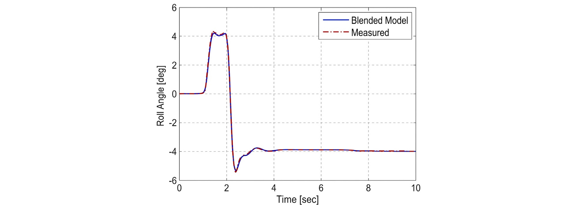
Estimating the roll angle by integrating the roll angular velocity accumulates integration errors over time, leading to significant errors. To reduce these errors, the integral is replaced by a pseudo-integrator with a low-pass filter applied. However, accurate estimation is difficult in low-frequency steady-state conditions because the integration result decreases rapidly. Therefore, an estimation method was applied that appropriately combined the kinematic-based Eq. (15), accurate at low frequency, and the Eq. (16), accurate at high frequency.

(17)

w (s) = \frac{b_{b l}}{s + b_{b l}}

In Eq. (17), $w (s)$ is a frequency-dependent weighting function, which is a Laplace domain function with $b_{b l}$ as a filter parameter. It approaches 0 at high frequencies and approaches 1 at low frequencies. The roll angle estimation combined using this function can be defined as in Eqs. (18)-(19).

(18)

ϕ_{e b l} = w (s) ϕ_{e k} + [1 - w (s)] ϕ_{e w}

(19)

ϕ_{e b l} = \frac{b_{b l}}{s + b_{b l}} ϕ_{e k} + \frac{s}{s + b_{b l}} ϕ_{e w}

In Eqs. (15)-(19), $ϕ_{e k}$ is the kinematic roll-angle estimate [rad], $ϕ_{e w}$ is the roll-angle estimate obtained by integrating the measured roll rate [rad], and $ϕ_{e b l}$ is the blended roll-angle estimate [rad]. The variable $τ$ denotes the integration variable [s], $s$ is the Laplace variable [s⁻¹], $b_{b l}$ is the filter break frequency [rad/s], and $w (s)$ is a dimensionless frequency-dependent weighting function. All angular calculations are performed in radians, and the results are converted to degrees only for presentation in Fig. 9. The simulation results obtained using this blended estimator are shown in Fig. 9.

https://cdn.apub.kr/journalsite/sites/kasa/2026-018-03/N0380180306/images/kasa_18_03_06_F9.jpg

Fig. 9

Roll angle estimation using combined model

3.2. Rollover Index

To maximize the performance of the active suspension control function, additional control strategies were implemented under rollover conditions.^(7,⁸⁾ To assess rollover risk, an energy-based rollover index was defined and utilized as a criterion for rollover determination.

Fig. 10 illustrates the behavior of a vehicle undergoing roll. For a vehicle to overturn, a corresponding amount of lateral and rotational kinetic energy is required. Therefore, by calculating the kinetic energy, the potential for overturning can be determined and defined using Eq. (20) – Eq. (22).

https://cdn.apub.kr/journalsite/sites/kasa/2026-018-03/N0380180306/images/kasa_18_03_06_F10.jpg

Fig. 10

Vehicle body rollover situation

(20)

R_{1} = \frac{ϕ}{\sin^{- 1} (\frac{T}{2 h})}

(21)

R_{2} = \frac{I {\dot{ϕ}}^{2}}{m_{s} g (\sqrt{4 h^{2} + T^{2}} - T \sin (2 ϕ) - \sqrt{T^{2} \sin^{2} ϕ + 4 h^{2} \cos^{2} ϕ})}

(22)

I = I_{C G} + m_{s} {(T \tan ϕ + \frac{\sqrt{T^{2} \sin^{2} ϕ + 4 h^{2}}}{2})}^{2}

Using the same frequency-dependent weighting function as that employed for roll-angle estimation, the blended rollover index is calculated from Eq. (23).

(23)

R_{b l} = R_{1} w (s) + R_{2} [1 - w (s)]

In Eqs. (20)-(23), $R_{1}$ is the roll-angle-based rollover index, $R_{2}$ is the rotational-energy-based rollover index, and $R_{b l}$ is the blended rollover index; all three indices are dimensionless. The quantities $T$ and $h$ denote the vehicle track width and sprung-mass center-of-gravity height, respectively [m], while $m_{s}$ is the sprung mass [kg]. The variables $ϕ$ and $\dot{ϕ}$ are the roll angle [rad] and roll rate [rad/s], respectively, and $g$ is gravitational acceleration [m/s²]. The quantities $I_{C G}$ and $I$ denote the sprung-body roll moment of inertia about its center of gravity and the effective moment of inertia about the rollover axis, respectively [kg·m²]. The weighting function $w (s)$ is dimensionless and is identical to that defined in Eq. (17). All geometric quantities listed in millimeters in Tables 4 and 5 are converted to meters before evaluating Eqs. (20)-(23). A rollover-index value approaching unity indicates that the vehicle is approaching the nominal rollover threshold defined by the adopted model.

Table 4.

Vehicle model parameters (SUV)

Vehicle	E-Class SUV: High CG
Suspension type	Independent-Solid axle
Parameter	Symbol	Value
Spring constant	K_s (F/R)	46/46 N/mm
Sprung mass	m_s	1592 kg
Unsprung mass	m_u	270 kg
CG height	h	1000 mm
Roll Center	R_x	621 mm
Track width	T	1575 mm
Wheel base	L	2590 mm

Table 5.

Vehicle model parameters (Sedan)

Vehicle	E-Class Sedan
Suspension type	Independent- Independent
Parameter	Symbol	Value
Spring constant	K_s (F/R)	34/46 N/mm
Sprung mass	m_s	1653 kg
Unsprung mass	m_u	180 kg
CG height	h	590 mm
Roll Center	R_x	609 mm
Track width	T	1600 mm
Wheel base	L	3048 mm

4. Simulation Results

4.1. Rollover Simulation

All vehicle-dynamics simulations were performed using CarSim-Simulink co-simulation. A flat, dry-asphalt road with a friction coefficient of $μ$ = 0.85 and the standard nonlinear tire model provided in CarSim were used. Identical road and tire settings were maintained for the active- and passive-suspension cases. The controller was updated at a fixed sampling time of $T_{s}$ = 10 ms, which was also used as the co-simulation communication step.

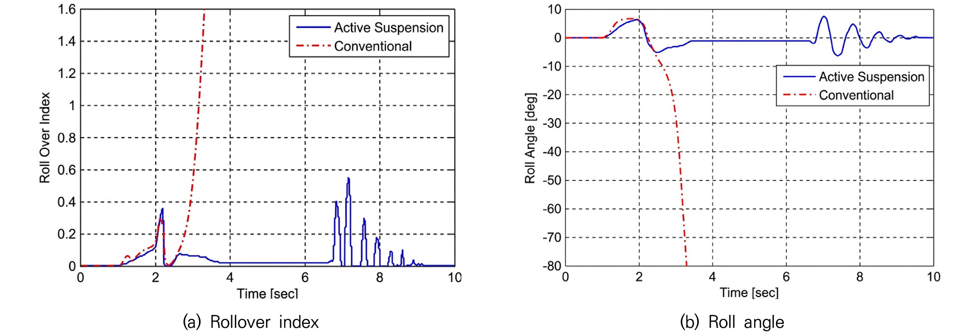
The rollover simulations followed the NHTSA fishhook steering sequence (9). The vehicle entered the maneuver at 50 mph (approximately 80 km/h) with the throttle released. The reference angle $δ_{0.3 g}$ was defined as the steering-wheel angle required to produce a steady-state lateral acceleration of 0.3 g at 50 mph. The steering wheel was ramped at 720°/s to +6.5 $δ_{0.3 g}$ and held for 0.25 s. It was then reversed at 720°/s through a total angle of 13 $δ_{0.3 g}$ to -6.5 $δ_{0.3 g}$ , held at that angle for 3.0 s, and returned to 0° within 1.0 s. The active- and passive-suspension cases received the identical steering command, and each fishhook run was simulated for 10 s.

Rollover was judged to occur when the blended rollover index defined in Eq. (23) reached or exceeded unity, $R_{b l}$ ≥ 1.0. The same threshold was applied to all vehicle and suspension configurations; rapid divergence of the roll-angle response was used as supporting confirmation of the rollover state.

The simulation procedure was set to fishhook, a scenario representing roll behavior simulation with an initial speed of 80 km/h.

As shown in Fig. 11(a)-(b), the passive car rolled over in approximately 3.2 seconds. On the other hand, it was confirmed that when equipped with active suspension, rollover was prevented while maintaining a roll angle of less than 5 degrees. Therefore, for vehicles with high ground clearance, such as SUVs, the effectiveness of active roll control during sudden lane changes, such as collision avoidance, can be considered significant. To further verify performance in a standard passenger car, the same simulation was performed using a model of the E-Class Sedan.

https://cdn.apub.kr/journalsite/sites/kasa/2026-018-03/N0380180306/images/kasa_18_03_06_F11.jpg

Fig. 11

Rollover index and roll angle (SUV)

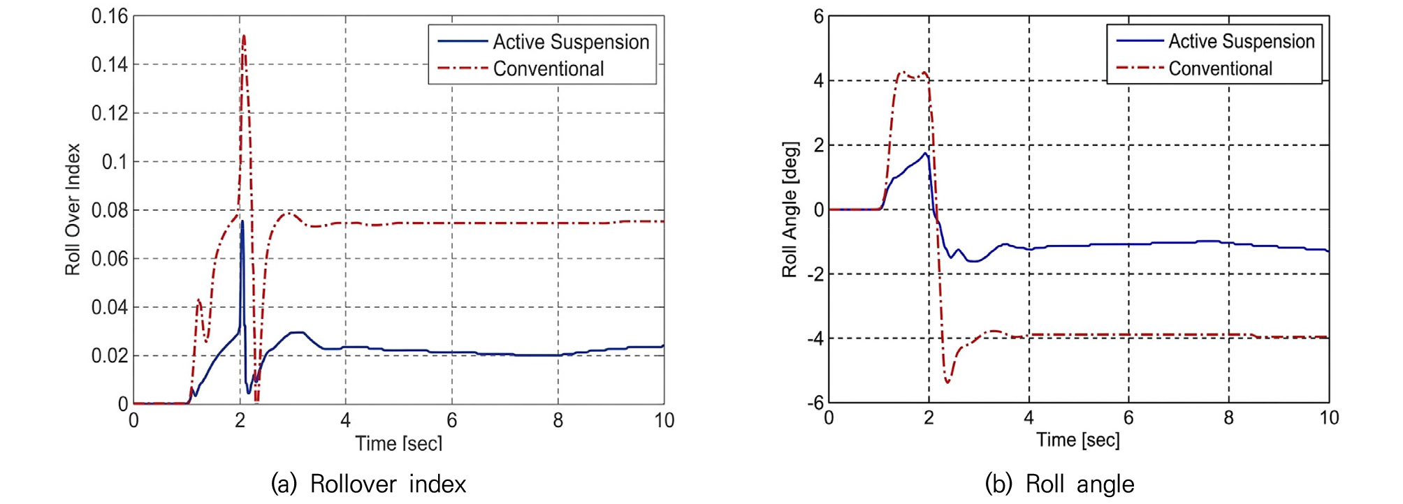
As shown in Fig. 12(a)-(b), the rollover index and roll angle decreased by more than 70% for vehicles equipped with active suspension compared to passive vehicles. Therefore, the effectiveness of active roll control using an active suspension actuator is demonstrated by assessing rollover risk in driving situations, such as sudden lane changes or collision avoidance, in passenger cars.

https://cdn.apub.kr/journalsite/sites/kasa/2026-018-03/N0380180306/images/kasa_18_03_06_F12.jpg

Fig. 12

Rollover index and roll angle (Sedan)

4.2. Dynamic Maneuver Simulation

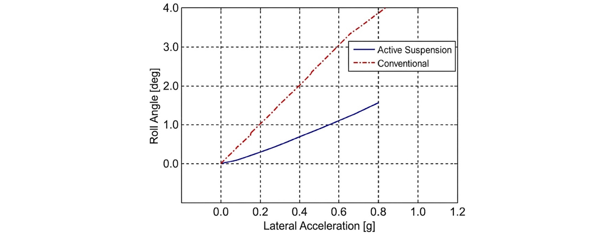
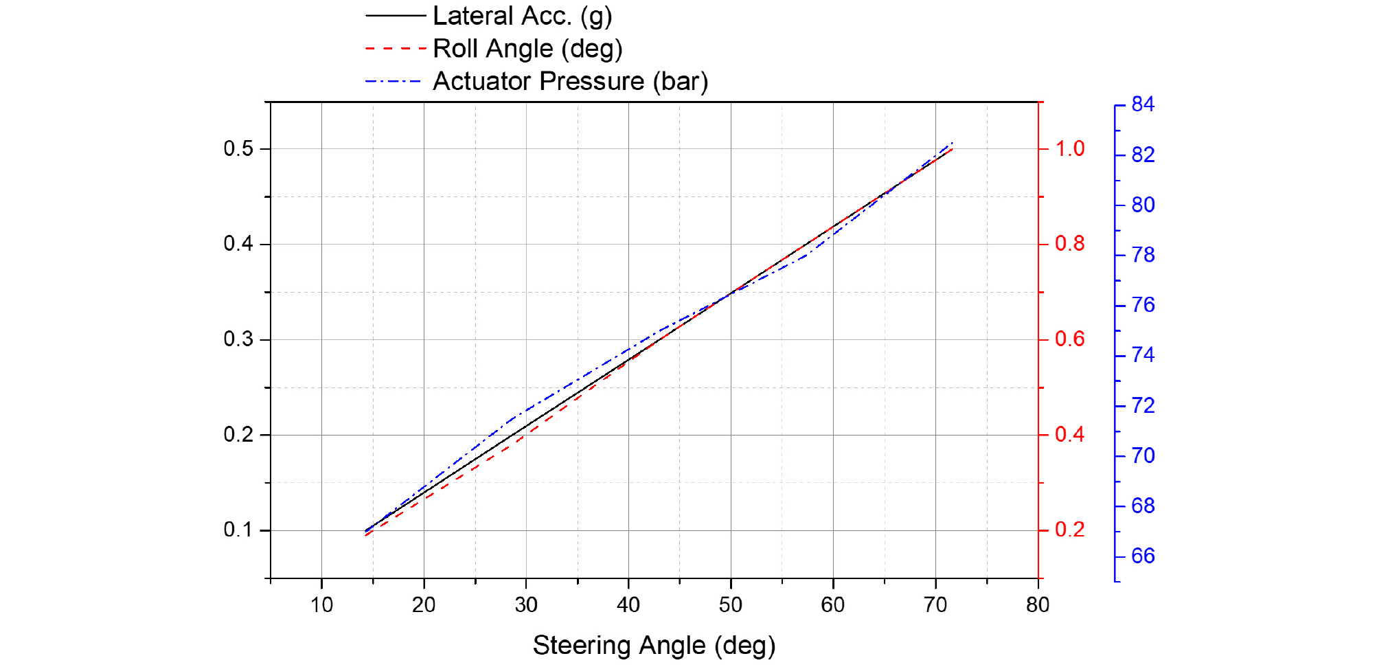
The dynamic steering simulations were conducted with the E-Class Sedan at an initial vehicle speed of 80 km/h under the same dry-asphalt road, CarSim tire-model, and sampling-time conditions described above. A standardized open-loop steering procedure was used to determine the actuator load and to derive system design requirements. The active-suspension performance target was a roll angle of 1° or less at a lateral acceleration of 0.5 g. The controller gain was adjusted to satisfy this target, and the resulting roll-angle-versus-lateral-acceleration relationship is shown in Fig. 13.

https://cdn.apub.kr/journalsite/sites/kasa/2026-018-03/N0380180306/images/kasa_18_03_06_F13.jpg

Fig. 13

Vehicle roll angle vs. lateral acceleration

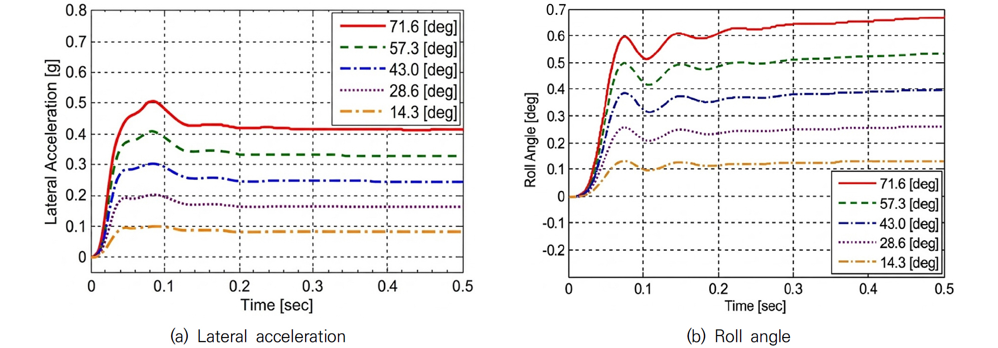
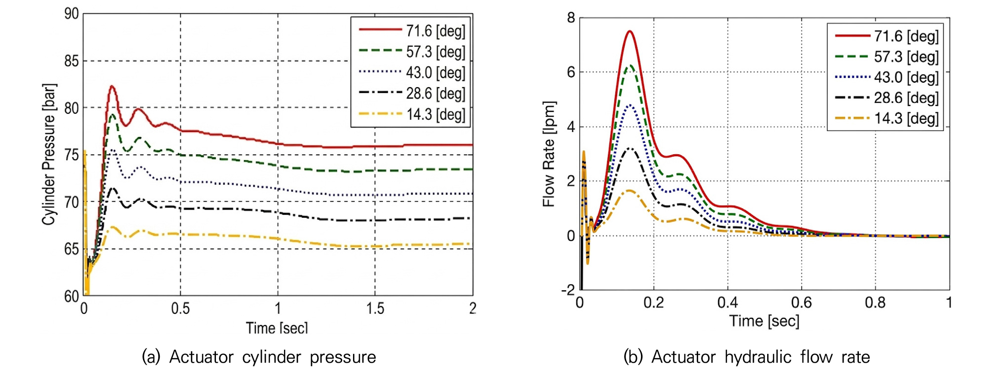
Five separate steering-wheel step inputs of 14.3°, 28.6°, 43.0°, 57.3°, and 71.6° (0.25, 0.50, 0.75, 1.00, and 1.25 rad, respectively) were applied and held until the vehicle response approached a quasi-steady condition. These input levels were selected to generate staged lateral-acceleration conditions up to approximately 0.5 g. For each input, the lateral acceleration, roll angle, actuator cylinder pressure, and hydraulic flow rate were evaluated using identical initial and environmental conditions. The input-dependent vehicle and actuator responses are shown in Figs. 14 and 15, respectively.

Fig. 14(a) shows the lateral acceleration response under different steering input conditions. As the steering angle increased, lateral acceleration increased in discrete steps. Under each condition, the system tended to converge to a relatively stable quasi-steady state following an initial transient response. This implies that the lateral load conditions used to evaluate control performance and actuator requirements were appropriately derived from the steering input.

Fig. 14(b) shows the roll-angle response under the same steering-input conditions. Although the roll angle increased with lateral acceleration, it remained within a limited range across all conditions without diverging excessively. In particular, even with large steering inputs, the roll angle response was suppressed to approximately 1 degree or less, confirming that the proposed active suspension-based roll control can effectively reduce vehicle body roll even under high lateral acceleration.

https://cdn.apub.kr/journalsite/sites/kasa/2026-018-03/N0380180306/images/kasa_18_03_06_F14.jpg

Fig. 14

Vehicle motion according to steering input conditions

Under the 0.5 g condition, the maximum simulated actuator cylinder pressure was 82.5 bar and the quasi-steady pressure was approximately 80 bar, while the transient peak flow rate was approximately 7.5 L/min, as shown in Fig. 15(a)-(b). The simulated maximum was rounded upward to 85 bar to define the peak operating-pressure requirement used for preliminary actuator sizing and for the simplified energy-demand comparison below.

https://cdn.apub.kr/journalsite/sites/kasa/2026-018-03/N0380180306/images/kasa_18_03_06_F15.jpg

Fig. 15

Actuator dynamics under different steering input conditions

For an indicative comparison with a conventional system that maintains a 200-bar supply, the hydraulic input power and energy are expressed as $P_{h} = p_{s} q_{c}$ and $\int p_{s} q_{c} d t$ , respectively. If the same flow demand, displaced fluid volume, and pressure-source efficiency are assumed, the energy ratio is approximated by $E_{h, p r o p} / E_{h, 200} \approx p_{p r o p} /$ (200 bar). At the representative peak condition of $p_{p r o p}$ = 85 bar and $q_{c}$ = 7.5 L/min, the proposed pressure demand corresponds to approximately 1.06 kW, compared with 2.50 kW at 200 bar for the same flow. The pressure-related peak hydraulic-power demand is therefore 57.5% lower. At the 80-bar quasi-steady pressure, the corresponding pressure-proportional hydraulic-energy reduction per unit displaced fluid volume is 60.0%.

Fig. 15(b) also shows that substantial flow is required mainly during the initial transient and approaches zero after approximately 0.6 s. This operating characteristic supports on-demand pressure generation rather than continuous high-pressure operation. However, the present model does not include motor-pump efficiency maps, internal leakage, accumulator behavior, or a representative driving-cycle duty ratio. The calculated 57.5-60.0% values therefore represent a simplified pressure-related hydraulic-energy potential and should not be interpreted as a measured full-system electrical-energy saving.

Among the actuator design parameters, the maximum allowable cylinder pressure ( $P_{m a x}$ ), initial cylinder pressure ( $p_{c, 0}$ ), effective hydraulic area ( $A_{e}$ ), and suspension spring stiffness ( $k_{s}$ ) have a direct influence on the system performance. The maximum cylinder pressure and effective hydraulic area determine the actuator force capacity according to ( $F_{m a x} = P_{m a x} A_{e}$ ). However, the initial cylinder pressure changes the pressure difference across the control valve and consequently affects the hydraulic flow rate and actuator response, as described in Eqs. (9)–(11). In addition, for a given hydraulic flow rate, the piston velocity is approximately inversely proportional to the effective hydraulic area, ( $\dot{x} = q_{c} / A_{e}$ ). Therefore, increasing the effective area improves the force capacity for a given pressure but requires a larger flow rate to achieve the same stroke response.

The spring stiffness is also an important design parameter because the present active suspension employs a series-type configuration. The actuator does not directly apply the control force to the sprung mass; instead, it generates the control force by changing the spring deformation. Accordingly, the change in spring force is related to the actuator displacement by ( $∆ F_{s} = k_{s} ∆ x_{a}$ ). These parameters should therefore be considered together to balance the required load capacity, hydraulic pressure, flow demand, response time, and actuator stroke.

When designing an electric motor for use in a motor pump, torque and RPM specifications must be selected based on the maximum internal pressure and flow rate required to meet the target specifications. In addition, appropriate gear strength and ratios must be considered to ensure the durability of all gears, including torque-transmitting components, rack bars, and pinions. The force exerted by the piston can be verified using Eq. (24).

The maximum pressure in Fig. 15(a) occurred for the largest steering input, which generated the target lateral acceleration of approximately 0.5 $g$ . The exact simulated peak, $p_{p e a k}$ = 82.5 bar, was therefore taken as the operating load point. For conservative preliminary load sizing, the effective hydraulic area measured in Table 3, 7.960 cm², was rounded downward to the nominal value $A_{e, n o m}$ = 7.9 cm². The pressure-to-force conversion is given in Eq. (24), where 1 kgf = 9.80665 N.

(24)

F_{o p} = p_{p e a k} A_{e, n o m} = (82.5 \times 10^{5} P a) (7.9 \times 10^{- 4} m^{2}) = 6517.5 N \approx 664.6 k g f

Accordingly, 664.6 kgf is the required operating load associated with the simulated peak condition; it is not the rated force corresponding to the 100 bar design pressure. The peak operating-pressure requirement was set to 85 bar by rounding the 82.5 bar simulation result upward to the nearest 5 bar. A practical design rating of $p_{d e s i g n}$ = 100 bar was then selected. This corresponds to a pressure margin of 100/85 ‒ 1 = 17.6% above the rounded operating requirement, or 100/82.5 ‒ 1 = 21.2% above the exact simulated peak. This preliminary margin allows for pressure fluctuations, modeling uncertainty, and control overshoot; it is not a substitute for the component-level structural safety factor required in detailed hardware design. At 100 bar and $A_{e, n o m}$ = 7.9 cm², the theoretical hydraulic force is 7900 N, or approximately 805.6 kgf. Therefore, the pressure-containing actuator components should be rated for at least 100 bar, and the mechanical load path should be checked against the corresponding design-pressure force.

https://cdn.apub.kr/journalsite/sites/kasa/2026-018-03/N0380180306/images/kasa_18_03_06_F16.jpg

Fig. 16

Lateral acceleration, roll angle, and actuator pressure versus steering angle

5. Conclusion and Future Work

This study verified the effectiveness of an electro-hydraulic active suspension system under emergency driving conditions, including rollover-critical scenarios. In addition, the actuator requirements for maintaining the target roll angle were systematically investigated from a control-oriented system design perspective.

For active roll control, the pressure source must generate the required cylinder pressure and flow rate within a short response time. Therefore, the driving motor should be sized to provide sufficient torque and rotational speed for the target roll-control performance. However, simply increasing motor capacity is not a practical solution because it may increase system costs and energy consumption. Accordingly, the actuator and motor specifications should be determined by considering the required roll-control performance, hydraulic pressure, flow rate, structural load, and system efficiency under representative driving conditions. In particular, the maximum cylinder pressure, initial operating pressure, effective hydraulic area, and spring stiffness should be treated as coupled design parameters when determining the specifications of a series-type electro-hydraulic active suspension. Under the 0.5 g condition, the simplified equal-flow comparison indicates a 57.5% lower pressure-related peak hydraulic-power demand than the 200-bar reference and a 60.0% lower pressure-proportional energy demand at the 80-bar quasi-steady pressure. These values quantify the pressure-demand advantage but do not represent full-system electrical-energy consumption.

Future work will include detailed actuator modeling to support component-level sizing of the motor, pump, valve, piston-cylinder assembly, and mechanical transmission. This will enable more practical specification development for electro-hydraulic active suspension systems.

References

Tseng, H. E., and Hrovat, D., 2015, State of the art survey: active and semi-active suspension control, Vehicle system dynamics, 53(7), 1034-1062.

10.1080/00423114.2015.1037313

Karnopp D, Crosby M, Harwood R. Vibration control using semi-active force generators, J Manuf Sci Eng. 1974; 96(2): 619~626.

10.1115/1.3438373

Yue C, Butsuen T, Hedrick JK. Alternative control laws for automotive active suspensions, In American Control Conference; 1988 June 15~17; Atlanta, GA.

10.23919/ACC.1988.4790124

Yu, M., Evangelou, S. A., and Dini, D., 2024, “Advances in active suspension systems for road vehicles,” Engineering, 33, 160-177.

10.1016/j.eng.2023.06.014

Guido Koch, 2011, “Actuator Control for a Hybrid Suspension System,” Technical Reports on Automatic Control, Vol. TRAC-6, 1~14.

Koch, G., Fritsch, O., and Lohmann, B., 2010, “Potential of low bandwidth active suspension control with continuously variable damper,” Control Engineering Practice, 18(11), 1251~1262.

10.1016/j.conengprac.2010.03.007

Hanlong Yang and Louis Yizhang Liu, 2003, “A Robust Active Suspension Controller with Rollover Prevention,” SAE 2003 Congress, 2003-01-0959, 1~6.

10.4271/2003-01-0959

Aleksander Hac, David Nichols, and Daniel Sygnarowicz, 2010, “Estimation of Vehicle Roll Angle and Side Slip for Crash Sensing,” SAE 2010 Congress, 2010-01-0529, 1~13.

10.4271/2010-01-0529

National Highway Traffic Safety Administration (NHTSA), 2013, “Dynamic Rollover Resistance (Fishhook Maneuver) Test Procedure,” New Car Assessment Program (NCAP), U.S. Department of Transportation.

Journal of Auto-vehicle Safety Association ISSN:2005-9396(Print) 자동차안전학회지

Preview

Electro-Hydraulic Active Suspension for Rollover Prevention: Control Performance and Actuator Design Requirements

ABSTRACT

MAIN

Fig. 1

Active suspension quarter-car model

(1)

(2)

(3)

Fig. 2

Schematic of the hydraulic actuator and valve

Fig. 3

Block diagram of the hydraulic actuator

(4)

(5)

(6)

(7)

(8)

Table 1.

Parameters of the reference hydraulic actuator model (Ref. 5)

(9)

(10)

(11)

Fig. 4

Response performance of the actuator displacement

Table 2.

Response time of the actuator’s linear motion

Fig. 5

Active suspension actuator test setup

Fig. 6

Actuator minimum (left) & maximum (right) stroke

Fig. 7

Actuator displacement according to hydraulic pressure

Table 3.

Experimentally identified parameters of the commercial actuator

(12)

(13)

(14)

Fig. 8

Vehicle Roll Motion Coordinates

(15)

(16)

(17)

(18)

(19)

Fig. 9

Roll angle estimation using combined model

Fig. 10

Vehicle body rollover situation

(20)

(21)

(22)

(23)

Table 4.

Vehicle model parameters (SUV)

Table 5.

Vehicle model parameters (Sedan)

Fig. 11

Rollover index and roll angle (SUV)

Fig. 12

Rollover index and roll angle (Sedan)

Fig. 13

Vehicle roll angle vs. lateral acceleration

Fig. 14

Vehicle motion according to steering input conditions

Fig. 15

Actuator dynamics under different steering input conditions

(24)

Fig. 16

Lateral acceleration, roll angle, and actuator pressure versus steering angle

References