Robust Path Tracking Control of an E-Corner Vehicle under Nonlinear Tire Dynamics Using Soft Actor-Critic

Eun-jin Jang; Jae-poong Lee; Hee-seung Lim

doi:10.22680/kasa2026.18.1.099

Preview

Journal of Auto-vehicle Safety Association. 31 March 2026. 99-109
https://doi.org/10.22680/kasa2026.18.1.099

Robust Path Tracking Control of an E-Corner Vehicle under Nonlinear Tire Dynamics Using Soft Actor-Critic

Eun-jin Jang¹^*

Jae-poong Lee²^†

Hee-seung Lim³

¹Undergraduate, Dept. of Intelligent Systems & Robotics, Chungbuk National University

²Assistant Professor, Dept of Intelligent Systems & Robotics, Chungbuk National University

³Senior Research Engineer, Electrification Research Team, Seohan Innobility

^{*First Author}

^{†Corresponding Author}

ABSTRACT

This paper aims to design a robust path tracking controller for E-Corner vehicles operating under environmental uncertainties and varying driving conditions. To this end, we build a vehicle dynamics simulation incorporating the Fiala tire model with a compact parameter set to capture realistic lateral tire behavior. A steering policy is then trained using Soft Actor-Critic, an off-policy reinforcement learning algorithm that maximizes both expected return and policy entropy, thereby promoting robust exploration and stable learning in continuous action spaces. The entropy-regularized objective of SAC enables the policy to remain resilient to modeling uncertainties and variations in vehicle dynamics, which are critical in path tracking tasks under diverse operating conditions. The vehicle model adopts a steering configuration that includes both front-wheel steering and rear-wheel steering to improve yaw rate tracking performance during path tracking maneuvers. Simulation results show that the learned agent maintains stable tracking performance under various conditions, achieving a yaw rate tracking error as low as 0.0023 rad/s at a vehicle speed of 20 m/s. In particular, a policy trained under a weave scenario also exhibits stable path tracking performance when deployed on trajectories acquired from the KIAPI Proving Ground, indicating good transferability beyond the training conditions and improved robustness to unseen path profiles.

Keywords

Reinforcement learning

Path tracking

Soft actor-critic

Nonlinear tire model

E-corner

MAIN

1. Introduction
2. Vehicle Modeling
2.1. Definition of Slip Angles
2.2. Vertical Load Model
2.3. Fiala Lateral Force Model
2.4. Steering Model
2.5. Definition of Lateral Acceleration and Yaw Rate
2.6. Substep Based Integration
3. Reinforcement Learning Environment
3.1. Reinforcement Learning Framework
4. Scenario Design and Results
4.1. Scenario Design
4.2. Results
5. Conclusion

1. Introduction

Path tracking, a core function of autonomous vehicles, involves controlling steering to precisely follow a designated path. Especially during high-speed maneuvers or on paths with high curvature, steering inputs lead to significant changes in vehicle attitude. Furthermore, uncertainties exist as vehicle responses vary depending on driving speeds, even under identical control inputs. In environments characterized by such nonlinearities and uncertainties, it is challenging to ensure consistent performance and stability across all driving conditions using only linearization-based models or fixed-gain control methods. Therefore, this study employs reinforcement learning algorithms, which can learn control policies through interactions across diverse conditions and operate stably even in the presence of model uncertainties.

To account for nonlinear tire dynamics, this study constructs a vehicle dynamics model based on the Fiala tire model,⁽¹⁾ which utilizes a relatively small number of parameters. Additionally, to enhance yaw rate tracking performance, a steering architecture incorporating both front-wheel and rear-wheel steering is applied. This configuration aims to reduce errors relative to the target yaw rate and ensure more stable path tracking performance. Furthermore, the front-and-rear steering structure adopted in this study is designed with future extensibility to E-Corner vehicle platforms—which include four-wheel independent steering⁽²⁾ and driving—in mind. This provides a foundation for RL policies to integrally learn the interactions between control inputs even in environments with the expanded degrees of freedom provided by corner modules.

In this study, the Soft Actor-Critic⁽³⁾ algorithm, an off-policy method, is applied to train the yaw rate tracking policy, ensuring stable learning and high sample efficiency in continuous control problems. SAC promotes exploration and enhances convergence stability during the training process through an entropy-regularized objective function that simultaneously maximizes expected rewards and policy entropy. This induces a robust policy capable of handling uncertain environments and dynamic variations. Consequently, this study aims to design a robust path tracking controller that minimizes yaw rate tracking errors and maintains stability under various driving conditions.

2. Vehicle Modeling

In this study, the vehicle dynamics model employs a vehicle mass of 1500 kg, a yaw moment of inertia of 2250 $k g \cdot m^{2}$ , and distances from the center of gravity to the front and rear axles of 1.2 m and 1.6 m, respectively. The tire cornering stiffness is set to 80,000 N/rad, and the road friction coefficient is assumed to be 0.8.

2.1. Definition of Slip Angles

In this study, a bicycle model is assumed, where the front and rear wheels of the vehicle are modeled as a single equivalent tire each. The front and rear slip angles are defined using the vehicle's lateral velocity $v_{y}$ , yaw rate $r$ , longitudinal velocity $v_{x}$ , and the respective steering angles $δ_{f}$ and $δ_{r}$ . The front slip angle $α_{f}$ is defined as in Eq. (1), and the rear slip angle $α_{r}$ is defined as in Eq. (2).

(1)

α_{f} = \arctan (\frac{v_{y} + l_{f} r}{v_{x}}) - δ_{f}

(2)

α_{r} = \arctan (\frac{v_{y} - l_{f} r}{v_{x}}) - δ_{r}

2.2. Vertical Load Model

The vertical loads acting on the front and rear wheels are defined using a static distribution model that neglects dynamic load transfer. The vertical load for the front wheels is expressed in Eq. (3), and for the rear wheels in Eq. (4).

(3)

F_{z f} = \frac{m g l_{r}}{l_{f} + l_{r}}

(4)

F_{z r} = \frac{m g l_{f}}{l_{f} + l_{r}}

2.3. Fiala Lateral Force Model

In this study, a brush-based⁽⁴⁾ Fiala tire model was employed to incorporate the nonlinear lateral force characteristics occurring at the tire-road contact patch into the vehicle model. This model has the advantage of representing the nonlinear variations in lateral force as the slip angle increases, as well as the saturation behavior caused by friction limits, in a relatively concise form. Furthermore, it enables modeling with a smaller number of parameters⁽⁵⁾ compared to other complex tire models. Through this approach, we aimed to ensure both computational efficiency and physical validity required for training the reinforcement learning-based controller.

The lateral forces of the front and rear tires were calculated using the Fiala model, taking each tire's slip angle and vertical load as inputs. When the slip angle is below a critical threshold $α_{s a t}$ , the lateral force is expressed as shown in Eq. (5).

(5)

F_{y} = - C_{α} \tan α + \frac{C_{α}^{2}}{3 μ F_{z}} |\tan α| \tan α - \frac{C_{α}^{3}}{27 μ^{2} F_{z}^{2}} \tan^{3} α

The critical slip angle $α_{s a t}$ is defined as shown in Eq. (6)

(6)

|α| \leq α_{s a t} = \arctan (\frac{3 μ F_{z}}{C_{α}})

When the slip angle exceeds the critical threshold, the tire lateral force saturates at the friction limit.

2.4. Steering Model

In this study, a second-order steering dynamics model was employed, where the steering input is defined as the steering angular acceleration $\ddot{δ}$ . This input is integrated to update the steering angular velocity $\dot{δ}$ and the steering angle $δ$ , as expressed in Eq. (7) and Eq. (8), respectively.

(7)

{\dot{δ}}_{k + 1} = {\dot{δ}}_{k} + {\ddot{δ}}_{k} ∆ t

(8)

δ_{k + 1} = δ_{k} + {\dot{δ}}_{k + 1} ∆ t

2.5. Definition of Lateral Acceleration and Yaw Rate

The vehicle's lateral acceleration ${\dot{v}}_{y}$ and yaw acceleration $\dot{r}$ are defined as shown in Eq. (9) and Eq. (10), respectively.

(9)

{\dot{v}}_{y} = \frac{F_{y f} \cos (δ_{f}) + F_{y r} \cos (δ_{r})}{m} - v_{x} r

(10)

\dot{r} = \frac{l_{f} F_{y f} \cos (δ_{f}) - l_{r} F_{y r} \cos (δ_{r})}{I_{z}}

The state updates for the lateral velocity and yaw rate are expressed in Eq. (11) and Eq. (12), as follows

(11)

v_{y} = v_{y} + {\dot{v}}_{y} ∆ t

(12)

r = r + \dot{r} ∆ t

2.6. Substep Based Integration

To mitigate numerical instability that may occur when performing a single integration over a large time interval, this study conducted numerical integration by dividing each environment step into five sub-steps.

The sub-step-based numerical integration allows for the stable application of steering angle and steering angular velocity constraints over more granular time intervals. Furthermore, it provides a more continuous and stable simulation of the process through which nonlinear tire lateral forces are transmitted to the yaw rate and lateral acceleration responses.

3. Reinforcement Learning Environment

3.1. Reinforcement Learning Framework

3.1.1. Soft Actor-Critic

Soft Actor-Critic is an off-policy actor-critic reinforcement learning algorithm suitable for continuous control problems. In this framework, the actor outputs a stochastic action $a$ for a given state $s$ , while the critic learns by approximating the action-value function $Q (s, a)$ . The core of SAC lies in its entropy-regularized objective function, which promotes exploration⁽⁶⁾ and enhances learning stability⁽⁷⁾ by maximizing not only the expected cumulative reward but also the entropy of the policy. The entropy-regularized objective function of SAC is defined as shown in Eq. (13).

(13)

J (π) = E [\sum_{t} (r (s_{t}, a_{t}) + α H (π (\cdot | s_{t})))]

In Eq. (13), $H (π (\cdot | s_{t}))$ denotes the entropy of the policy, and $α$ serves as a temperature parameter that adjusts the weighting of the entropy term, thereby balancing the trade-off between exploration and exploitation. Furthermore, SAC enhances sample efficiency by reusing past experiences through a replay buffer.⁽⁸⁾ It also ensures learning stability by employing clipped double-Q learning to mitigate the overestimation of Q-values.⁽⁹⁾

The objective of this study is to train a steering policy capable of ensuring stable path tracking performance even in environments characterized by nonlinear tire dynamics,⁽¹⁰⁾ as described by the Fiala tire model. In such environments, responses to state-action changes can vary sensitively due to the nonlinearity of tire lateral forces. This poses a risk where the policy might prematurely converge to a suboptimal solution or the learning process could become unstable without sufficient exploration.

Reinforcement learning-based control offers the advantage of directly learning the relationships between states, actions, and rewards for these nonlinear systems without the need for explicit model linearization or complex control rule design. While traditional rule-based controller design becomes increasingly difficult as interactions between control inputs grow more complex—particularly in multi-degree-of-freedom control problems—RL enables integral policy learning even within high-dimensional state and action spaces.

Consequently, this study applies the SAC algorithm, which maintains exploration through entropy regularization while performing stable training based on off-policy learning and the double-Q structure. By maintaining the stochastic nature of the policy, SAC secures the ability to explore various driving conditions while simultaneously improving learning stability and data efficiency.

Moreover, the front-and-rear steering configuration considered in this study is intended for future extensibility to E-Corner vehicle platforms, which feature four-wheel independent steering and driving. In such E-Corner-based vehicles, the action space expands significantly due to independent control over each wheel, and the coupling effects between control inputs become highly complex. RL-based control is a particularly suitable approach for vehicle platforms with expanded degrees of freedom, as it can integrally learn these interactions within the policy, even in large action spaces. Thus, this study aims to train a robust yaw rate and path tracking control policy that accounts for both nonlinear tire dynamics and the potential for future expansion to E-Corner platforms through SAC-based reinforcement learning.

3.1.2. Configuration of the Reinforcement Learning Environment

In this study, the SAC algorithm is employed to train a steering policy for yaw rate tracking. The states, actions, and rewards of the reinforcement learning framework are configured to ensure optimal path tracking performance. The specific observations and actions used in the training process are summarized in Table 1.

Table 1.

Components of SAC learning

Type	Feature	Units
Observation	Lateral velocity Longitudinal velocity Yaw rate Front wheel steering angle Front wheel steering rate Rear wheel steering angle Rear wheel steering rate Target yaw rate Yaw rate tracking error	m/s m/s rad/s rad rad/s rad rad/s rad/s rad/s
Action	Front steering angular acceleration Rear steering angular acceleration	rad/s² rad/s²

First, the lateral velocity and yaw rate were included in the observations as they directly influence yaw rate tracking performance and vehicle stability. Next, the steering angles and steering angular velocities of the front and rear wheels were incorporated. These are essential internal states since the system follows a second-order steering dynamics model where the input is defined as steering angular acceleration; including them allows the policy to consider actual steering responses and the proximity to steering constraints.

The target yaw rate provides the reference to be followed at the current time step, while the tracking error serves as direct error feedback representing the control objective, contributing to both learning convergence and tracking precision. Finally, the longitudinal velocity was included to allow the policy to calculate appropriate steering inputs adapted to varying speed conditions.

The final output of the reinforcement learning agent is defined as the steering angular accelerations for the front and rear wheels. By directly controlling the rate of change of the steering input, the policy learns to mitigate discontinuous vehicle responses caused by abrupt steering maneuvers and achieves smooth steering control within the defined constraint boundaries.

3.1.3. Reward Function Design

In this study, the reward function was designed as a weighted sum of a tracking term and a stability term to simultaneously account for yaw rate tracking performance and lateral stability. First, the tracking error term is formulated as shown in Eq. (14).

(14)

R_{t r a c k i n g} = e x p (- k_{r} |e_{r}|)

The reward associated with the magnitude of the lateral velocity $v_{y}$ , which is related to lateral stability, is structured as in Eq. (15).

(15)

R_{s t a b i l i t y} = e x p (- k_{v} |v_{y}|)

The final reward is composed as a weighted sum of these two terms, as shown in Eq. (16), prioritizing tracking performance while also reflecting stability.

(16)

R_{m i x} = w_{r} R_{t r a c k i n g} + (1 - w_{r}) R_{s t a b i l i t y}

Furthermore, to normalize the reward range for more effective learning, a linear transformation was applied to define the final step reward as in Eq. (17).

(17)

R = 2 R_{m i x} - 1

Based on the previously described sub-step integration, the reward for a single environment step is determined by averaging the rewards calculated at each sub-step, as expressed in Eq. (18).

(18)

R_{s t e p} = \frac{1}{N} \sum_{i = 1}^{N} R^{(i)}

Finally, regarding the termination conditions, an episode is terminated and a large negative reward is assigned if the lateral velocity increases excessively or the yaw rate tracking error exceeds a certain threshold, signifying a failure state. This approach prevents the policy from entering unstable lateral states or divergent tracking conditions, guiding the learning process toward achieving stable yaw rate tracking.

3.1.4. Training Parameters

The SAC training parameters used in this study are summarized in Table 2.

Table 2.

SAC training parameters

Parameter	Value
Optimizer	Adam
Learning rate	3·10^-4
Discount factor	0.95
Replay buffer size	10⁶
Number of hidden layers	2
Number of hidden nodes	256
Activation function	ReLU
Batch size	256

3.1.5. Normalization

In this study, the observations were normalized to enhance the stability and convergence speed of the reinforcement learning process. Since the scales of the physical quantities in the observations vary significantly, gradient scale imbalances can occur during neural network training. To prevent this, all observation values were divided by predefined scale constants before being input into the network. The normalization scale constants used are summarized in Table 3 below.

Table 3.

Normalization statistics of observations

Feature	Scale
Lateral velocity [m/s]	2.0
Longitudinal velocity [m/s]	15.0
Yaw rate [rad/s]	1.0
Front steering angle [rad]	0.5236
Front steering rate [rad/s]	1.5708
Rear steering angle [rad]	0.5236
Rear steering rate [rad/s]	1.5708
Reference yaw rate [rad/s]	1.0
Yaw rate tracking error [rad/s]	0.3

3.1.6. Training Conditions

In this study, to train the reinforcement learning-based yaw rate tracking policy, a training environment was configured where the driving conditions and target yaw rate inputs are randomized for each episode. This approach ensures that the agent encounters a wide range of scenarios, thereby improving the robustness and generalization of the learned policy across diverse operational conditions.

At the start of each episode, a target yaw rate input scenario is randomly selected as either a sinusoidal or a ramp function. The parameters of the selected profile are randomly sampled from the ranges specified in Table 4 and Table 5. The selected scenario remains fixed throughout the duration of that specific episode. This configuration induces the policy to learn robust tracking performance across various types of target yaw rate trajectories.

Table 4.

Yaw rate reference conditions for sine profiles

Sinusoidal yaw rate
Amplitude [rad/s]	0.01-0.25
Frequency [Hz]	0.02-1.0
Velocity [m/s]	9-21

Table 5.

Yaw rate reference conditions for ramp profiles

Ramp yaw rate
Slope [rad/s²]	0.1-0.3
Maximum value [rad/s]	0.01-0.25
Velocity [m/s]	9-21

4. Scenario Design and Results

4.1. Scenario Design

In this study, to ensure the stable performance of the agent, the policy was trained to track a sine-wave target yaw rate under various training conditions. The evaluation scenarios for yaw rate tracking were designed by categorizing the sine-wave target yaw rate tracking, as detailed in Table 6, into two distinct speed conditions.

Table 6.

Yaw rate tracking scenario conditions

Case 1: Yaw rate tracking
Velocity [m/s]	10	20
Frequency [Hz]	0.2
Amplitude [rad/s]	0.1

To quantitatively verify the agent's performance, including stability during the yaw rate tracking process, we selected the target yaw rate tracking error, front and rear steering angles, and lateral velocity as the primary evaluation metrics.

In addition, to evaluate the generalization performance of the policy trained on sine-wave and ramp-type target yaw rates, a path was constructed as shown in Fig. 1 using road data acquired from the KIAPI Proving Ground. The evaluation scenario was conducted under a constant speed condition of 20 m/s, as detailed in Table 7.

https://cdn.apub.kr/journalsite/sites/kasa/2026-018-01/N0380180108/images/kasa_18_01_08_F1.jpg

Fig. 1

KIAPI proving ground visualization

Table 7.

Path tracking scenario conditions

Case 2: Path tracking
Velocity [m/s]	20

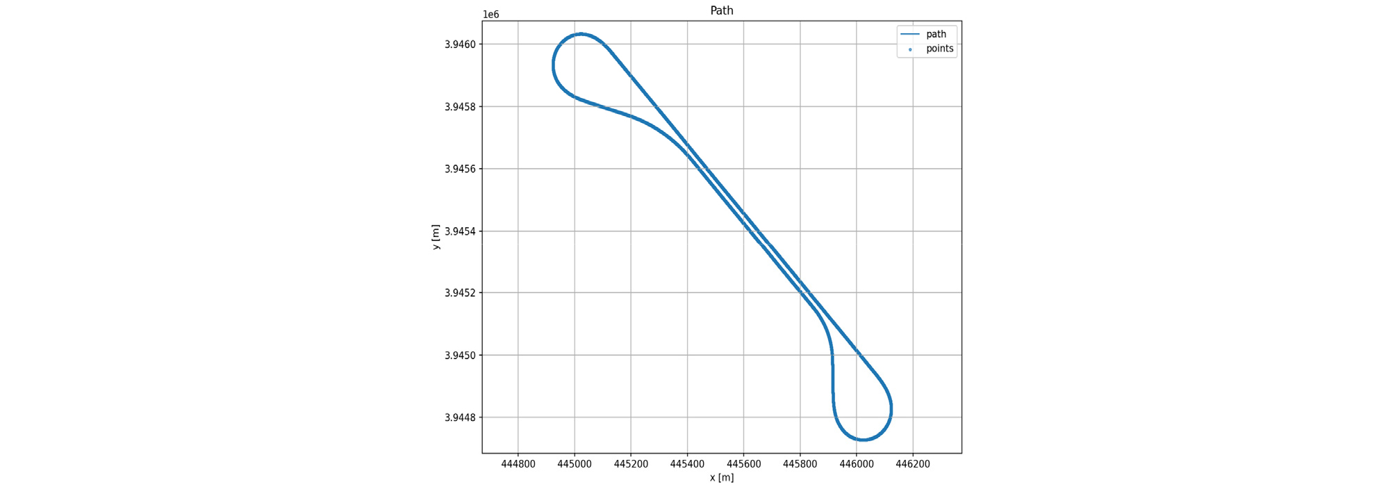
The target curvature was calculated by applying the Pure Pursuit algorithm to the x and y coordinates of the centerline extracted from the road data. Subsequently, the target yaw rate was generated by combining this curvature with the vehicle's longitudinal velocity.

4.2. Results

4.2.1. Case 1: Target Yaw Rate Tracking

The simulation results for the constant speed conditions of 10 m/s and 20 m/s are presented in Fig. 2 and Fig. 3, respectively.

https://cdn.apub.kr/journalsite/sites/kasa/2026-018-01/N0380180108/images/kasa_18_01_08_F2.jpg

Fig. 2

Yaw rate tracking performance at 10 m/s under a weave test

https://cdn.apub.kr/journalsite/sites/kasa/2026-018-01/N0380180108/images/kasa_18_01_08_F3.jpg

Fig. 3

Yaw rate tracking performance at 20 m/s under a weave test

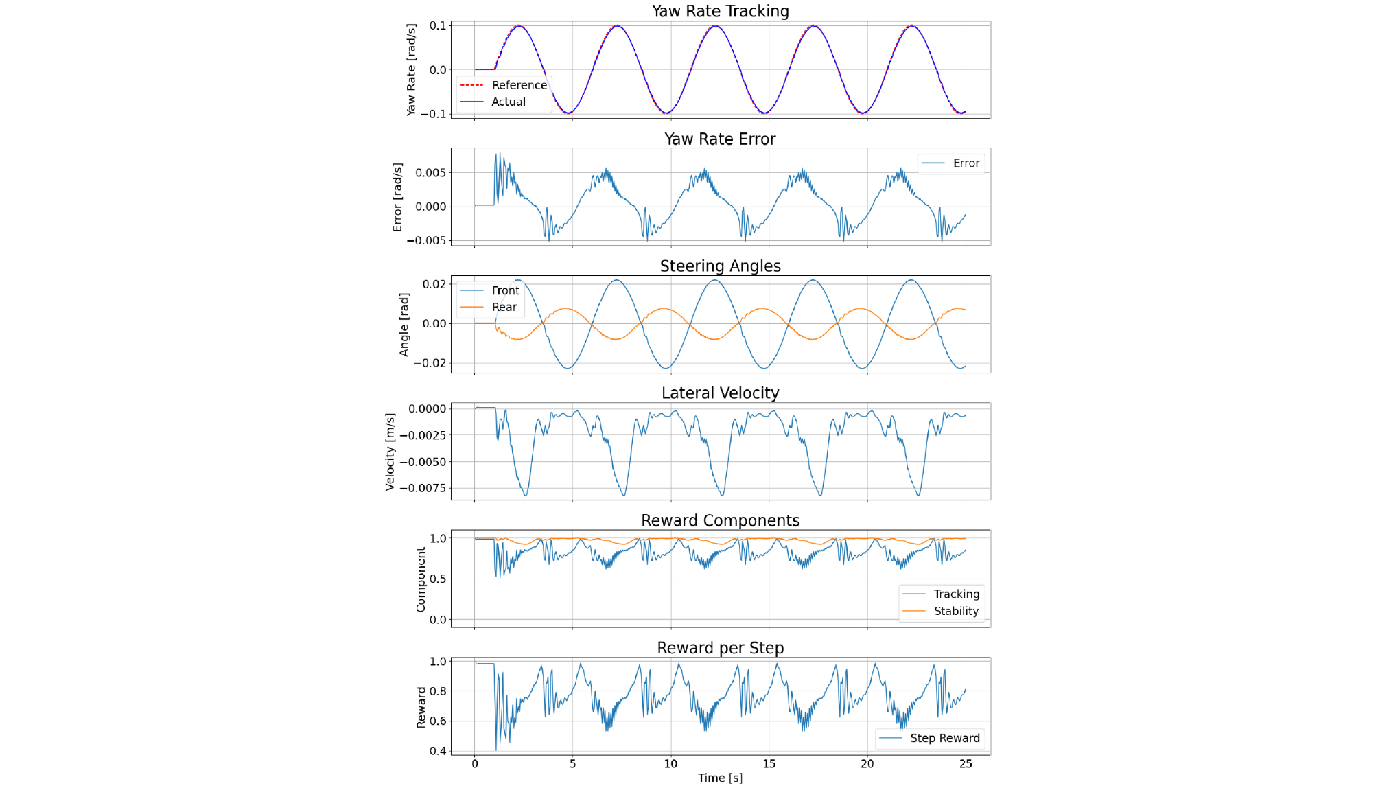
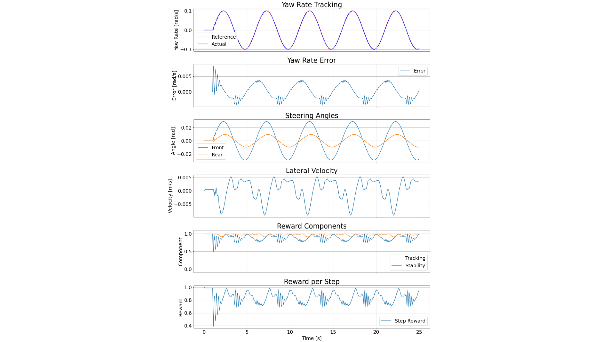
The yaw rate tracking errors for each speed condition are summarized in Table 8.

Table 8.

Yaw rate tracking performance evaluation results

velocity [m/s]	10	20
Yaw rate error [rad/s]	0.0028	0.0023

The experimental results confirm that for both 10 m/s and 20 m/s constant speed conditions, the yaw rate tracking error was maintained near zero. Furthermore, the reward was observed to converge stably, indicating improvements in both tracking performance and vehicle stability.

4.2.2. Case 2: Path Tracking

The path tracking performance of the agent at a constant speed of 20 m/s is illustrated in Fig. 4 and Fig. 5.

https://cdn.apub.kr/journalsite/sites/kasa/2026-018-01/N0380180108/images/kasa_18_01_08_F4.jpg

Fig. 4

Zoomed-in view of path tracking performance in the high curvature section of the KIAPI proving ground

https://cdn.apub.kr/journalsite/sites/kasa/2026-018-01/N0380180108/images/kasa_18_01_08_F5.jpg

Fig. 5

Path tracking performance at 20 m/s on the KIAPI proving ground

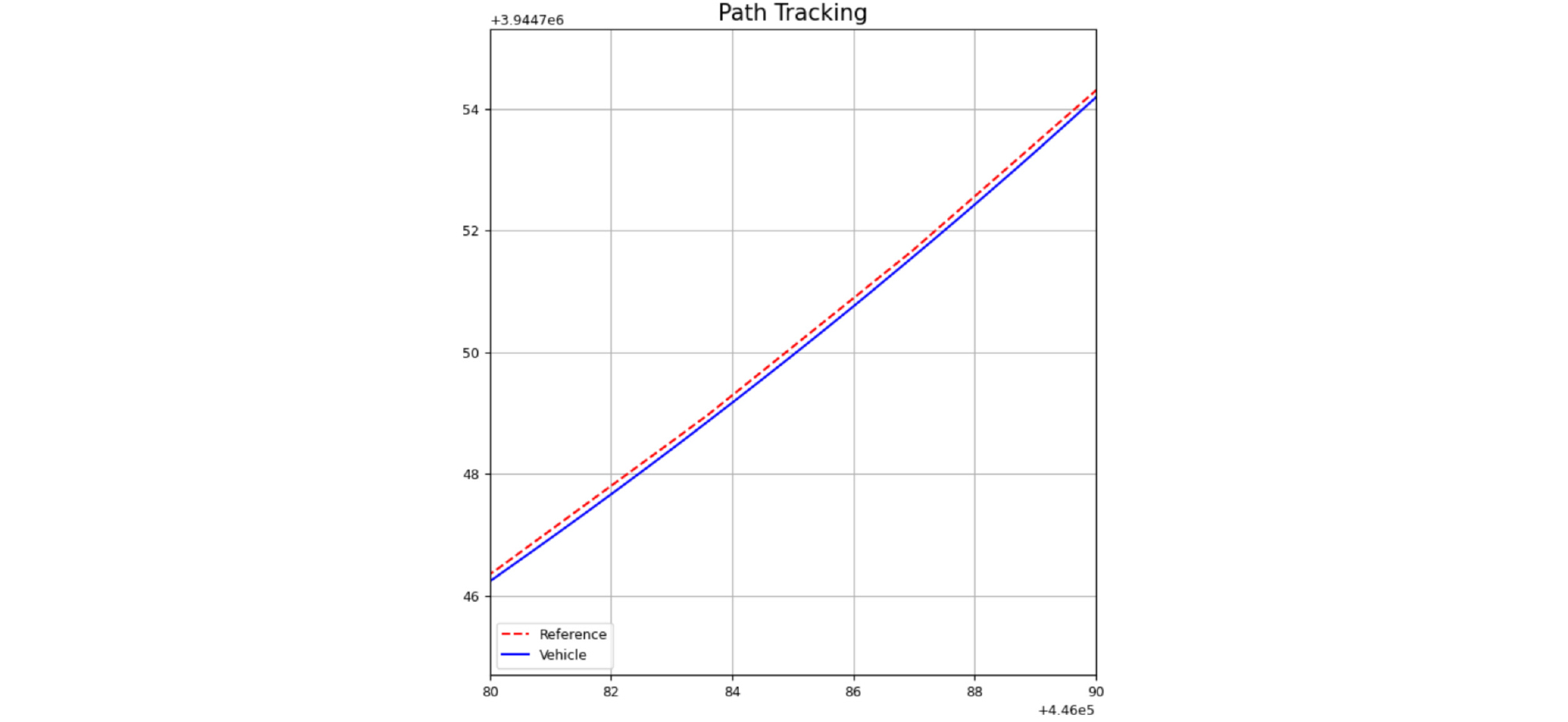
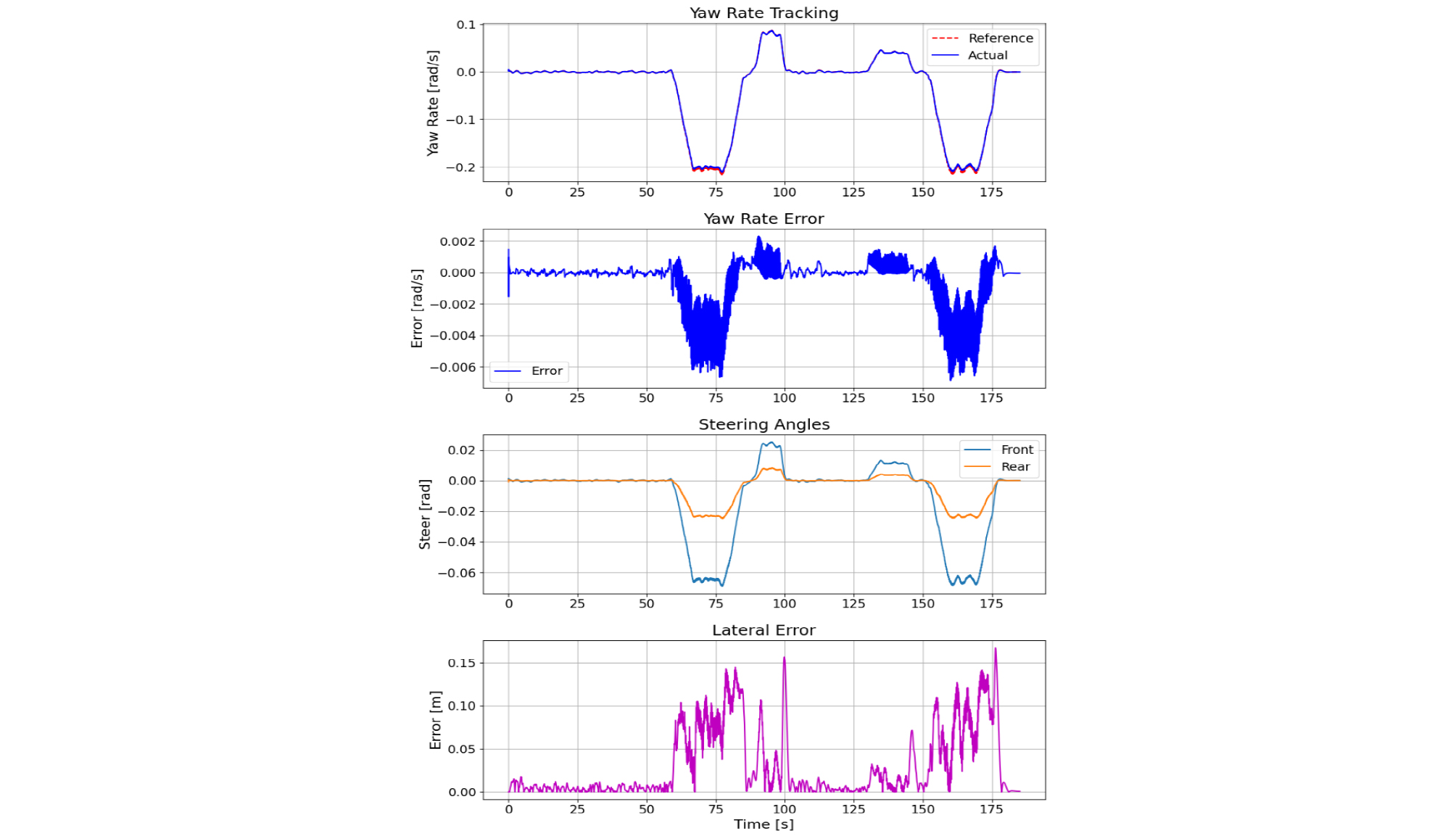
The path tracking performance metrics at a constant speed of 20 m/s are presented in Table 9.

Table 9.

Path tracking performance evaluation results

velocity [m/s]	20
Lateral RMSE [m]	0.0507
Maximum lateral error [m]	0.1676

The experimental results demonstrated that the agent maintained the lateral error near zero, confirming that the target yaw rate was tracked accurately during path tracking.

5. Conclusion

In this study, a reinforcement learning-based path tracking controller was developed to ensure stable tracking performance even under conditions where tire lateral forces exhibit nonlinear behavior relative to slip angles. To this end, a vehicle dynamics model was constructed by applying the brush-based Fiala tire model, which effectively captures tire saturation characteristics with a minimal set of parameters. For the control policy, the Soft Actor-Critic (SAC) algorithm was employed to simultaneously secure exploration and learning stability within a continuous control framework. The steering input was generated based on a front-and-rear steering configuration, a structure designed with future extensibility to E-Corner vehicle platforms—incorporating four-wheel independent steering and driving—in mind. Furthermore, by dividing each environment step into multiple sub-steps, the effects of steering dynamics and nonlinear tire forces on yaw rate and lateral error were simulated more stably and accurately.

Simulation results confirmed that the policy, trained to follow sine-wave target yaw rates, achieved stable tracking across various speed conditions. Moreover, when the trained policy was applied to target yaw rates generated via Pure Pursuit using road coordinates from the KIAPI Proving Ground, stable path tracking was maintained even for path geometries not encountered during the training phase. These results demonstrate that the learned control policy possesses a significant degree of generalization and robustness across diverse path conditions, rather than being limited to specific scenarios.

Future work will build upon the front-and-rear steering policy structure established in this study to incorporate the additional degrees of freedom offered by E-Corner vehicles. This expansion aims to achieve even more robust path tracking control under a broader range of complex driving conditions.

Acknowledgements

This research was supported by the Regional Innovation System & Education (RISE) program through the (Chungbuk Regional Innovation System & Education Center), funded by the Ministry of Education (MOE) and the (Chungcheongbuk-do), Republic of Korea. (2025-RISE-11-014-03)

References

Fiala, E., 1954, “Lateral Forces on Rolling Pneumatic Tires,” Zeitschrift VDI, Vol. 96, No. 973, pp. 973~979.

Yim, S., 2020, “Comparison among Active Front, Front Independent, 4-Wheel and 4-Wheel Independent Steering Systems for Vehicle Stability Control,” Electronics, Vol. 9, No. 5, pp. 798~798.

10.3390/electronics9050798

Haarnoja, T., Zhou, A., Abbeel, P., and Levine, S., 2018, “Soft Actor-Critic: Off-Policy Maximum Entropy Deep Reinforcement Learning with a Stochastic Actor,” International Conference on Machine Learning (ICML), pp. 1861~1870.

Pacejka, H., 2005, Tire and Vehicle Dynamics, Elsevier, Oxford, UK, pp. 61~89.

10.1016/B978-075066918-4/50002-2

Viani, T., 2019, “LFT Parameter Identification of the Cornering Stiffnesses Based on the Fiala Tire Model,” Master’s Thesis, Politecnico di Milano, Milano, Italy, pp. 1~89.

Levine, S., 2018, “Reinforcement Learning and Control as Probabilistic Inference: Tutorial and Review,” arXiv preprint arXiv:1805.00909.

Haarnoja, T., Tang, H., Abbeel, P., and Levine, S., 2017, “Reinforcement Learning with Deep Energy-Based Policies,” International Conference on Machine Learning (ICML), pp. 1352~1361.

Mnih, V., et al., 2015, “Human-Level Control through Deep Reinforcement Learning,” Nature, Vol. 518, No. 7540, pp. 529~533.

10.1038/nature14236

Fujimoto, S., Hoof, H., and Meger, D., 2018, “Addressing Function Approximation Error in Actor-Critic Methods,” International Conference on Machine Learning (ICML), pp. 1587~1596.

Kebbati, Y., et al., 2023, “Lateral Control for Autonomous Wheeled Vehicles: A Technical Review,” Asian Journal of Control, Vol. 25, No. 4, pp. 2539~2563.

10.1002/asjc.2980

Journal of Auto-vehicle Safety Association ISSN:2005-9396(Print) 자동차안전학회지

Preview

Robust Path Tracking Control of an E-Corner Vehicle under Nonlinear Tire Dynamics Using Soft Actor-Critic

ABSTRACT

MAIN

(1)

(2)

(3)

(4)

(5)

(6)

(7)

(8)

(9)

(10)

(11)

(12)

(13)

Table 1.

Components of SAC learning

(14)

(15)

(16)

(17)

(18)

Table 2.

SAC training parameters

Table 3.

Normalization statistics of observations

Table 4.

Yaw rate reference conditions for sine profiles

Table 5.

Yaw rate reference conditions for ramp profiles

Table 6.

Yaw rate tracking scenario conditions

Fig. 1

KIAPI proving ground visualization

Table 7.

Path tracking scenario conditions

Fig. 2

Yaw rate tracking performance at 10 m/s under a weave test

Fig. 3

Yaw rate tracking performance at 20 m/s under a weave test

Table 8.

Yaw rate tracking performance evaluation results

Fig. 4

Zoomed-in view of path tracking performance in the high curvature section of the KIAPI proving ground

Fig. 5

Path tracking performance at 20 m/s on the KIAPI proving ground

Table 9.

Path tracking performance evaluation results

Acknowledgements

References