Integrated 6-DOF Vehicle Dynamics Modeling and Simulation-Based Validation for 4-Corner Independent Driving Platforms

Yu-sun Kim; Jae-poong Lee; Young-seung Yu; Jae-geun Bang

doi:10.22680/kasa2026.18.1.080

Preview

Journal of Auto-vehicle Safety Association. 31 March 2026. 80-98
https://doi.org/10.22680/kasa2026.18.1.080

Integrated 6-DOF Vehicle Dynamics Modeling and Simulation-Based Validation for 4-Corner Independent Driving Platforms

Yu-sun Kim¹^*

Jae-poong Lee²^†

Young-seung Yu³

Jae-geun Bang³

¹B.S. Student, Department of Intelligent Systems and Robotics, Chungbuk National University

²Assistant Professor, Department of Intelligent Systems and Robotics, Chungbuk National University

³Senior Research Engineer, Electrification Research Team, Seohan Innobility

^{*First Author}

^{†Corresponding Author}

ABSTRACT

This paper presents the development of an integrated vehicle dynamics simulator for e-Corner systems and its validation using simulation-based reference data. The proposed simulator is built on a four-corner vehicle architecture, in which each wheel independently models driving, braking, steering, suspension, and tire dynamics, and is coupled with a six-degree-of-freedom (6-DOF) rigid vehicle body model to capture full vehicle motion. To reproduce vehicle roll, pitch, and vertical load distribution characteristics with sufficient physical fidelity, force and moment interactions among the body, suspension, and tire subsystems are explicitly formulated and numerically integrated in the time domain. An equivalent anti-roll mechanism is implemented using active suspension actuators, in which the anti-roll moment is generated from the left–right suspension stroke difference and distributed to each corner as vertical forces, enabling realistic roll suppression behavior. The developed simulator is validated through direct comparison with CarMaker reference data under identical driving conditions. Key dynamic responses, including roll angle, pitch angle, wheel normal forces, and longitudinal and lateral vehicle motions, are evaluated. The results show that the proposed model closely follows the trends of the reference data and accurately reproduces roll behavior and load transfer characteristics observed in the commercial simulator. In addition, diagonal driving enabled by the e-Corner architecture is analyzed as a representative unconventional maneuver. The proposed model consistently reproduces this motion without inducing yaw rotation, demonstrating its capability to represent the distinctive kinematic and dynamic characteristics unique to e-Corner vehicles. Overall, the proposed simulation framework provides a physically consistent and extensible basis for future studies on active suspension systems, advanced motion control strategies, and comprehensive vehicle dynamics analysis for next-generation mobility platforms.

Keywords

Vehicle dynamics

e-Corner system

6-degree-of-freedom model

Active suspension

MAIN

1. Introduction
2. Configuration of e-Corner Vehicle Dynamics Subsystems
2.1. Structural Characteristics of the e-Corner Vehicle and Definition of the Analysis Target
2.2. Configuration of Each Subsystem
3. Configuration of the Integrated Vehicle Dynamics Simulator
3.1. Vehicle Coordinate System and State Variable Definitions
3.2. Vehicle Body Dynamics Equations (6-DOF)
3.3. Active Anti-Roll Control Mechanism
4. Model Validation and Results Analysis
4.1. Validation Method and Comparison Conditions
4.2. Model Validation and Results Analysis
4.3. Validation of e-Corner-Specific Driving Motions
5. Conclusion

1. Introduction

With recent advances in vehicle propulsion and control technologies, e-Corner systems, in which each wheel independently performs driving, braking, steering, and suspension functions, have emerged as a next-generation vehicle platform. While this architecture provides high degrees of freedom and flexible motion control, it also increases the complexity of interactions among the vehicle body, suspension, and tires, making subsystem-based analysis insufficient for accurately describing overall vehicle behavior. Therefore, an integrated vehicle dynamics model that considers the entire vehicle is required to analyze the dynamic characteristics of e-Corner vehicles under diverse driving conditions.

Since each corner of an e-Corner vehicle includes independent actuators and dynamic components, conventional simplified vehicle models have limitations in reproducing actual body behavior.

Accordingly, a 6-degree-of-freedom (6-DOF) vehicle body dynamics model coupled with wheel-level driving, braking, steering, suspension, and tire dynamics is essential for comprehensive system-level analysis. This integrated approach enables systematic investigation of the effects of individual corner dynamics on vehicle motion.

CarMaker, a widely used commercial vehicle dynamics simulator, realistically models body roll behavior and wheel load distribution through suspension coupling effects, including a passive anti-roll bar. In contrast, e-Corner vehicles employ independent active suspension actuators at each wheel. In this study, an active suspension-based anti-roll mechanism is introduced to reproduce roll behavior and left–right coupling effects comparable to those of the CarMaker model.

This paper develops an integrated vehicle dynamics simulator for e-Corner systems and validates it using CarMaker simulation data. The proposed simulator is based on a four-corner vehicle architecture coupled with a 6-DOF vehicle body dynamics model and is evaluated under identical driving conditions in terms of roll angle, pitch angle, wheel vertical loads, and longitudinal and lateral vehicle motions. The results confirm that the proposed simulator provides a physically consistent and reliable framework for analyzing e-Corner vehicle architectures. Quantitative comparison against the CarMaker reference shows high agreement, with RMSEs of 1.2×10^-3 rad for pitch and 2.9×10^-3 rad for yaw, and correlations of 0.9899 and 0.9999, respectively.

2. Configuration of e-Corner Vehicle Dynamics Subsystems

2.1. Structural Characteristics of the e-Corner Vehicle and Definition of the Analysis Target

The e-Corner system is based on a vehicle architecture in which each wheel independently performs driving, braking, steering, and suspension functions, with individual actuators and dynamic elements arranged at each corner. As a result, wheel-level torques and forces directly act on the vehicle body. In such e-Corner vehicles, the longitudinal, lateral, and vertical tire forces generated at each corner significantly influence the translational and rotational motions of the vehicle body; therefore, an analysis framework that simultaneously considers corner-level dynamics and vehicle body motion is required. Accordingly, this study adopts an integrated analysis structure that couples wheel-level dynamic models with a vehicle body dynamics model to capture the coupled interactions among subsystems during transient vehicle maneuvers.

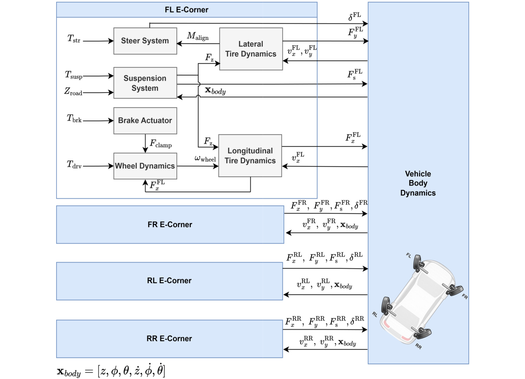
Fig. 1 illustrates the structure of the e-Corner vehicle considered in this study and provides an overview of the simulation configuration. The target vehicle consists of four independent corners, and the forces generated at each corner are transformed into forces and moments in the vehicle coordinate system and applied to the vehicle body to compute its time-domain dynamic response.

https://cdn.apub.kr/journalsite/sites/kasa/2026-018-01/N0380180107/images/kasa_18_01_07_F1.jpg

Fig. 1

Block diagram of the integrated 6-DOF vehicle dynamics simulator with e-Corner modules

2.2. Configuration of Each Subsystem

The e-Corner vehicle dynamics simulator developed in this study includes driving and braking, steering, active suspension, and tire models at each corner, which are coupled with a vehicle body dynamics model.

Each subsystem computes wheel-level forces or motion states from control inputs or body states, which are converted into forces and moments and applied to a 6-degree-of-freedom (6-DOF) vehicle body model. The resulting body states are fed back to each corner, forming a closed-loop vehicle dynamics analysis in the time domain.

To systematically present the e-Corner-based vehicle dynamics architecture, the input–state–output relationships of each corner-level subsystem are organized in Table 1. The table summarizes the signal definitions for the steering, driving/braking, suspension, and tire models, thereby clarifying the signal flow and coupling structure illustrated in Fig. 1. In particular, $T_{d r v}, T_{b r k}, T_{s t r}$ and $T_{s u s p}$ denote the actuator torque commands for traction, braking, steering, and suspension, respectively. The brake model outputs the clamping force $F_{c l a m p}$ (tracked from $F_{c l a m p}^{*}$ ) and wheel dynamics are represented by the wheel speed $w$ the suspension subsystem takes the road height input $Z_{r o a d}$ and unsprung states $(z_{u}, {\dot{z}}_{u})$ to produce the suspension force $F_{s}$ and tire vertical force $F_{z}$ , The tire model computes longitudinal/lateral forces $(F_{x}, F_{y})$ and aligning moment $M_{z}$ from wheel-frame velocities $(V_{w x}, V_{w y})$ , wheel speed $w$ , and $F_{z}$ , and these corner-level forces collectively drive the vehicle-body state $X_{b o d y}$ This section describes the configuration and functional roles of the corner subsystems and explains how their outputs contribute to vehicle-body motion based on the relationships summarized in Table 1.

Table 1.

I/O of the subsystems

Group	Component	Inputs	State	Outputs
Actuation	Brake Actuator	$T_{b r k}$	$F_{c l a m p}^{*}$	$F_{c l a m p}$
	Drive System	$T_{d r v}, F_{c l a m p}$	$w$	$w$
	Steer System	$T_{s t r}, T_{a l i g n}$	$δ, \dot{δ}$	$δ$
Suspension	Suspension System	$T_{s u s p}, Z_{r o a d}$	$z_{u}, {\dot{z}}_{u}$	$F_{s}, F_{z}$
Tire models	Longitudinal Tire Dynamics	$w, V_{w s}, F_{z}$	-	$F_{x}$
Tire models	Lateral Tire Dynamics	$V_{w x}, V_{w y}, F_{z}$	-	$F_{y}, M_{z}$
Vehicle body	Vehicle Body Dynamics	$F_{x}, F_{y}, F_{s}, δ$	$X_{b o d y}$	$X_{b o d y}, V_{w x}, V_{w y}$

Table 2.

Key vehicle specifications used in simulations

Category	Parameter	Unit	Value
Mass	Total mass	kg	2065.03
	Sprung mass		1806.80
	Unsprung mass (Front, per wheel)		74.12
	Unsprung mass (Rear, per wheel)		54.995
Geometry	Wheelbase	m	2.97
	Track width		1.634
	CG height		0.654
	CG to front axle distance		1.155
	CG to rear axle distance		1.815
Wheel/Tire	wheel radius		0.321
Inertia	Roll inertia	kg·m²	749.84
	Pitch inertia		2732.2
	Yaw inertia		2900.3

2.2.1. Driving and Braking Subsystem

The driving and braking subsystem determines the longitudinal vehicle behavior by converting the driving torque and braking inputs applied at each corner into the wheel rotational response. Considering the characteristics of the e-Corner vehicle architecture, this study constructs the driving and braking subsystem using a brake actuator model and a wheel dynamics model, and clearly defines the inputs, outputs, and state variables of each model.

The driving and braking subsystem consists of the brake actuator and the wheel dynamics model, and the two models are coupled in the time domain through their state variables. The brake actuator receives the braking input given as motor torque $T_{b r k}$ and generates a clamping force based on the hydraulic torque–pressure relationship and the pressure–clamping-force relationship.^(1,²⁾ The relationships between brake torque and hydraulic pressure, and between hydraulic pressure and clamping force $F_{c l a m p}$ , are expressed as follows.^(1,²⁾

(1)

T_{b r k} = \frac{∆ p V_{d}}{2 π}, F_{c l a m p} \approx 2 A_{e f f} p

where $T_{b r k}$ (N·m) is the brake actuator torque input, $∆ p$ (pa) is the pressure difference across the hydraulic actuator, $V_{d}$ (m³/rev) is the hydraulic displacement, $p$ (pa) is the brake line pressure, $A_{e f f}$ (m²) is the effective piston area, and $F_{c l a m p}$ (N) is the brake caliper clamping force. $V_{d}$ and $A_{e f f}$ were set from actuator specifications. By combining Eq. (1), the target clamping force corresponding to the brake torque input is formulated, and the brake response delay is incorporated as follows.⁽¹⁾

(2)

τ {\dot{F}}_{c l a m p} + F_{c l a m p} = F_{c l a m p, t a r g e t}

where $τ$ (s) is the brake actuator time constant representing response delay. $τ$ was selected as a representative value to reproduce stable and realistic brake transient behavior.^(3,⁴⁾

(3)

J_{w} \dot{w} = T_{d r v} - R_{e} F_{x} + M_{b r k} - B_{w} w

Where $J_{w}$ (kg·m²) is the equivalent wheel rotational inertia, $w$ (rad/s) is the wheel angular speed, $T_{d r v}$ (N·m) is the driving torque input, $R_{e}$ (m) is the effective rolling radius, $F_{x}$ (N) is the longitudinal tire force, $M_{b r k}$ (N·m) is the braking torque, and $B_{w}$ (N·m·s/rad) is an equivalent viscous rotational damping coefficient. $J_{w}$ and $R_{e}$ were set from wheel–tire geometry/specifications, and $B_{w}$ was set as a small positive constant. Eq. (3) is discretized to update the wheel angular velocity state $w$ , and the resulting response is used as input to the longitudinal tire model, enabling a consistent dynamic representation of wheel rotation and longitudinal force transmission.

2.2.2. Steering Subsystem

The steering actuator dynamics are described using a standard equivalent model commonly presented in the vehicle steering system modeling literature, as expressed below.^(5,⁶⁾

(4)

J_{e q} \ddot{δ} + B_{e q} \dot{δ} = T_{s t r} - T_{a l i g n}

Where, $δ$ (rad) denotes the tire steering angle at each corner, and $J_{e q}$ (kg·m²) and $B_{e q}$ (N·m·s/rad) represent the equivalent inertia and viscous damping coefficients corresponding to the steering motion. $T_{s t r}$ (N·m) is the corner-equivalent steering torque applied to the tire steering actuator, while $T_{a l i g n}$ (N·m) represents the self-aligning torque $M_{z}$ computed from the tire model.^(6,⁷⁾

2.2.3. Active Suspension Subsystem

The suspension subsystem models the vertical interaction between the vehicle body and the tire, and computes the tire vertical load and vehicle body response resulting from road inputs and variations in body attitude. In the e-Corner vehicle architecture, since the suspension at each corner operates independently, a model configuration that explicitly considers corner-level suspension dynamics is required. In this study, the corner-wise vertical positions of the vehicle body are calculated based on the heave, roll, and pitch motions obtained from the vehicle body model, and these positions are used to compute the suspension and tire vertical forces at each corner in the time domain. The unsprung-mass vertical dynamics are given as follows.^(8,⁹⁾

(5)

m_{u} {\ddot{z}}_{u} = F_{z} - F_{s} - m_{u} g

Where, $m_{u}$ (kg) is the unsprung mass, $z_{u}$ (m) is the absolute vertical position of the wheel center, $F_{z}$ (N) is the tire vertical force, $F_{s}$ (N) is the suspension force transmitted to the vehicle body, and $g$ (m/s²) is the gravitational acceleration. The suspension force is given as follows.

(6)

F_{s} = F_{s p r i n g} + F_{d a m p e r} + F_{a c t i v e}

Where $F_{s}$ is the suspension force, $F_{s p r i n g}$ (N) is the spring force, $F_{d a m p e r}$ (N) is the damper force, and $F_{a c t i v e}$ (N) is the active suspension force. The spring and damper forces are given as follows.

(7)

F_{s p r i n g} = - K_{s} δ_{s}, F_{d a m p e r} = - C_{s} {\dot{δ}}_{s}

Where $K_{s}$ (N/m) is the suspension spring stiffness, $C_{s}$ (N·s/m) is the suspension damping coefficient, $δ_{s}$ (m) is the suspension stroke, and ${\dot{δ}}_{s}$ (m/s) is the stroke velocity. The ball-screw actuator force–torque relation is given as follows.⁽¹⁰⁾

(8)

F_{a c t i v e} \approx \frac{2 π η}{l} T_{s u s p}

Where $T_{s u s p}$ (N·m) is the actuator input torque, $l$ (m/rev) is the screw lead, and $η$ (-) is the mechanical efficiency. The tire vertical force is given as follows.

(9)

F_{z} = K_{t} δ_{t} + C_{t} {\dot{δ}}_{t}

Where $K_{t}$ (N/m) is the tire vertical stiffness, $C_{t}$ (N·s/m) is the tire vertical damping coefficient, $δ_{t}$ (m) is the tire compression, and ${\dot{δ}}_{t}$ (m/s) is the compression velocity. The computed tire vertical force is used as an input for the vehicle body dynamics as well as for the calculation of longitudinal and lateral tire forces, enabling consistent time-domain coupling among road inputs, body attitude variations, and active suspension inputs.

2.2.4. Tire Model Subsystem

The tire subsystem computes the longitudinal force $F_{x}$ , lateral force $F_{y}$ , and self-aligning torque $M_{z}$ at each corner using the wheel local velocity and the vertical load $F_{z}$ . In this study, the adopted tire force model is a linear stiffness tire force model with friction-limited saturation, in which the linear force predictions are bounded by the friction constraint $μ F_{z}$ .⁽⁹⁾ This model was selected to ensure computational efficiency in time-domain simulation of the integrated 6-DOF vehicle dynamics while providing a clear baseline for validation, and the formulation is maintained in a modular form to allow future replacement or extension to higher-fidelity tire models when needed.⁽⁹⁾ In the wheel local reference frame, the slip angle is computed by

(10)

α = a t a n 2 (V_{m y}, V_{w x})

Where $α$ (rad) is the slip angle, and $V_{w x}$ (m/s) and $V_{w y}$ (m/s) are the longitudinal and lateral components of the wheel-center velocity in the wheel local frame.⁽⁹⁾ The corresponding lateral tire force is obtained using a linear cornering stiffness model and is limited by the friction constraint $μ F_{z}$

(11)

F_{y} = s a t (- C_{α}, - μ F_{z}, + μ F_{z})

Where $F_{y}$ (N) is the lateral tire force, $C_{α}$ (N/rad) is the cornering stiffness coefficient, $μ$ (-) is the road–tire friction coefficient, and $F_{z}$ (N) is the vertical load.^(10~¹²⁾ The self-aligning torque is approximated by

(12)

M_{z} = t_{p} F_{y}

Where $M_{z}$ (N·m) is the self-aligning torque and $t_{p}$ (m) is the trail.^(10~¹²⁾

For longitudinal motion analysis, the wheel circumferential velocity is defined as $V_{w h e e l} = w R_{e f f}$ , and the slip ratio is computed by

(13)

k = \frac{V_{w h e e l} - V_{w x}}{\max \{|V_{w x}|, V_{m i n}\}}

Where $k$ (-) is the slip ratio, $V_{w h e e l}$ (m/s) is the wheel circumferential speed, $w$ (rad/s) is the wheel angular speed, $R_{e f f}$ (m) is the effective radius, and $V_{m i n}$ (m/s) is a small positive threshold introduced to avoid division by near-zero speed.⁽¹¹⁾

The longitudinal tire force is calculated based on the linear stiffness coefficient and is similarly limited by the friction constraint $μ F_{z}$

(14)

F_{x} = s a t (C_{x} k, - μ F_{z}, + μ F_{z})

where $F_{x}$ (N) is the longitudinal tire force and $C_{x}$ (N) is the longitudinal stiffness coefficient.^(11~¹³⁾

The longitudinal and lateral tire forces and the aligning torque computed in this manner are used as inputs for the analysis of vehicle yaw and roll motions, as well as for the steering subsystem.⁽⁹⁾

3. Configuration of the Integrated Vehicle Dynamics Simulator

In the previous section, the steering, driving, braking, suspension, and tire subsystems of the e-Corner vehicle were modeled, and their input–output relationships were defined. This section describes the integration of these subsystems with rigid-body vehicle dynamics to construct a unified vehicle dynamics simulator.

Since the e-Corner vehicle generates forces independently at each wheel, the forces computed at each corner must be mapped to the translational and rotational motions of the vehicle body. Accordingly, the longitudinal and lateral tire forces and the vertical forces transmitted to the body are formulated as forces and moments acting on the vehicle body, and a six-degree-of-freedom (6-DOF) vehicle body dynamics model is derived.

The integrated model updates the vehicle body states in the time domain and feeds them back as kinematic inputs to each corner module, enabling consistent representation of the interactions between body motion and e-Corner modules. This section first defines the vehicle coordinate system and state variables, then presents the 6-DOF body dynamics equations and state update structure. In addition, an active suspension-based anti-roll mechanism is incorporated into the integrated model to reflect the structural characteristics of the e-Corner vehicle.

3.1. Vehicle Coordinate System and State Variable Definitions

For the mathematical formulation of vehicle dynamics, this study defines an inertial coordinate system, a vehicle body coordinate system, and a wheel coordinate system.

The inertial coordinate system $\{I\}$ is defined as a ground-fixed reference frame and is represented by $(X_{i}, Y_{I}, Z_{I})$ , where the $Z_{I}$ -axis is defined to point upward. The vehicle body coordinate system $\{B\}$ is fixed at the vehicle center of gravity (CG) and is represented by $(x, y, z)$ , with the x-axis pointing forward, the y-axis to the left, and the z-axis upward. The wheel coordinate system $\{W_{i}\}$ is defined at each corner $i \in \{F L, F R, R L, R R\}$ and is constructed as a coordinate frame rotated about the z-axis of the body coordinate system by the steering angle $δ_{i}$ .

(15)

η = {[ϕ, θ, ψ]}^{Τ}

As shown in Eq. (15), the vehicle body attitude is represented using ZYX-order Euler angles, which correspond to roll, pitch, and yaw angles, respectively.

(16)

v_{b} = {[u, v, w]}^{Τ}, w_{b} = {[p, q, r]}^{Τ}

The translational velocity and angular velocity of the vehicle body are defined in the body coordinate system as shown in Eq. (16). Accordingly, the integrated state vector of the vehicle is constructed as expressed in Eq. (17).⁽¹⁴⁾

(17)

X = {[\begin{matrix} P \\ η \\ v \\ w \end{matrix}]}^{Τ} = {[\begin{matrix} x & y & z \\ ϕ & θ & ψ \\ u & v & w \\ p & q & r \end{matrix}]}^{Τ}

Here, z is defined as a deviation coordinate (heave) with respect to the reference height, and the vertical motion of the vehicle body is computed by integrating this deviation coordinate. When the position vector of each corner with respect to the vehicle center of gravity is defined as $r_{i} = {[x_{i}, y_{i}, - h_{c g}]}^{Τ}$ , the velocity of each corner in the vehicle body coordinate system is calculated according to rigid-body kinematic relationships, as expressed in Eq. (18).

(18)

v_{b, i} = v_{b} + w_{b} \times r_{i}

In addition, the wheel coordinate system velocity considering the steering angle is obtained by rotating the vehicle body coordinate system velocity about the z-axis.

(19)

[\begin{matrix} V_{w x, i} \\ V_{w y, i} \end{matrix}] = R_{z} (- δ_{i}) [\begin{matrix} V_{b, i, x} \\ V_{b, i, y} \end{matrix}]

It is calculated as shown in Eq. (19). Here, $R_{z} (∙)$ denotes the rotation matrix about the z-axis, and the transformed velocity components are used to compute the tire slip angle and slip ratio at each corner.

3.2. Vehicle Body Dynamics Equations (6-DOF)

In this section, six-degree-of-freedom (6-DOF) vehicle body dynamics equations describing the translational and rotational motions of the vehicle body are presented based on the forces computed at each corner. Since each wheel in the e-Corner vehicle generates forces through independent actuators, it is necessary to formulate how the longitudinal tire forces, lateral tire forces, and vertical forces transmitted through the suspension at each corner are coupled to the rigid-body motion of the vehicle body.

Accordingly, the corner-level forces are assembled into resultant forces and moments in the vehicle body coordinate system and applied to the Newton–Euler equations. The longitudinal tire forces $F_{x, i}$ and lateral tire forces $F_{y, i}$ computed at each corner $i \in \{F L, F R, R L, R R\}$ are transformed into the vehicle body coordinate system by considering the steering angle $δ_{I}$ . The horizontal force components in the vehicle body coordinate system are defined as follows.

(20)

[\begin{matrix} F_{x, i}^{B} \\ F_{y, i}^{B} \end{matrix}] = R_{z} (δ_{i}) [\begin{matrix} F_{x, i}^{W} \\ F_{y, i}^{W} \end{matrix}]

Here, $R_{z} (∙)$ denotes the rotation matrix about the z-axis. The vertical force transmitted from each corner to the vehicle body is defined as the suspension force $F_{s, i}$ . Accordingly, the total force vector acting on the vehicle body is constructed as $F = {[F_{x}^{B}, F_{y}^{B}, F_{z}^{B}]}^{Τ}$ .

(21)

F = \sum_{i} [\begin{matrix} F^{B_{x, i}} \\ F^{B_{y, i}} \\ F_{s, i} \end{matrix}] + R {(η)}^{Τ} [\begin{matrix} 0 \\ 0 \\ - m_{s} g \end{matrix}]

Eq. (21) constructs the total force acting on the vehicle body by transforming and summing the horizontal forces generated at each corner into the vehicle body coordinate system and adding the vertical forces transmitted through the suspension. Since gravity is defined in the inertial coordinate system fixed to the ground, it is transformed into the vehicle body coordinate system and included in the total force. Here, $m_{s}$ denotes the sprung mass, and $R {(η)}^{Τ}$ represent the rotational transformation used to map the gravitational vector from the inertial coordinate system to the vehicle body coordinate system.

The moment vector about the vehicle center of gravity (CG) is defined as shown in Eq. (22).

(22)

M = {[M_{x}, M_{y}, M_{z}]}^{Τ}

The corner position vector $r_{i}$ represents the lever arm of each corner with respect to the vehicle center of gravity in the vehicle body coordinate system and is expressed as shown in Eq. (23).

(23)

r_{i} = {[x_{i}, y_{i}, - h_{c g}]}^{Τ}

The forces transmitted from each corner to the vehicle body act through these lever arms, generating roll, pitch, and yaw moments on the vehicle body.

In this study, roll and pitch motions are assumed to be primarily induced by the vertical force distribution at each corner; therefore, roll and pitch moments are formulated based on the points of application of the vertical forces. In contrast, the yaw moment is calculated from the in-plane horizontal forces acting on the vehicle body, as expressed in Eq. (24).

(24)

M_{x} = \sum_{i} y_{i} F_{s, i}, M_{y} = \sum_{i} (- x_{i}) F_{s, i}, M_{z} = \sum_{i} (x_{i} F_{y, i}^{B} - y_{i} F_{x, i}^{B})

In addition, longitudinal and lateral accelerations cause load redistribution with respect to the center-of-gravity height, which further influences roll and pitch motions. To account for this effect, an equivalent acceleration-proportional moment is defined as shown in Eq. (25).

(25)

M_{x, a c c} = M_{s} h_{c g} a_{y}, M_{y, a c c} = - m_{s} h_{c g} a_{x}

Here, $a_{x}$ and $a_{y}$ denote the longitudinal and lateral accelerations expressed in the vehicle body coordinate system, respectively. Using the forces and moments formulated in this manner, the translational and rotational motions of the vehicle body are described by the Newton–Euler equations given below.

(26)

m (\dot{V} + w \times V) = F, I \dot{w} + w \times (I w) = M + M_{a c c}

Here, $V = {[u, v, w]}^{Τ}$ represents the translational velocity of the vehicle body expressed in the body coordinate system, $w = {[p, q, r]}^{Τ}$ denotes the angular velocity of the vehicle body, and $I$ is the inertia tensor defined with respect to the vehicle center of gravity. Eq. (26) describes the rigid-body dynamics of the vehicle body, relating the forces generated at each corner to the longitudinal and lateral accelerations as well as the roll, pitch, and yaw motions of the vehicle body.⁽¹⁵⁾

3.3. Active Anti-Roll Control Mechanism

To reduce vehicle body roll motion, this study introduces an active anti-roll mechanism based on the operating principle of a conventional passive anti-roll bar (ARB). A passive ARB suppresses roll motion by generating a torsional moment proportional to the left–right suspension stroke difference; however, its characteristics are fixed by structural stiffness. In contrast, this study extends the same physical concept to an active approach that enables generation of a variable anti-roll moment through actuators.

The active anti-roll mechanism independently considers the front and rear axles, using the left–right suspension stroke difference at each axle as the input. The stroke differences for the front and rear axles are defined as follows.

(27)

∆ s_{f} = s_{F L} - s_{F R}, ∆ s_{r} = s_{R L} - s_{R R}

In Eq. (27), $S_{F L}, S_{F R}, S_{R L}, S_{R R}$ denotes the suspension stroke at each corner. The anti-roll moment generated at each axle is defined to be proportional to the stroke difference and its time derivative, in order to emulate the linear behavior of a passive anti-roll bar.

(28)

M_{a r b, f} = k_{a r b, f} ∆ s_{f} + c_{a r b, f} ∆ {\dot{s}}_{f}, M_{a r b, r} = k_{a r b, r} ∆ s_{r} + c_{a r b, r} ∆ {\dot{s}}_{r}

Here, $k_{a r b}$ and $c_{a r b}$ denote the anti-roll stiffness and damping coefficients, respectively, and are independently specified for the front and rear axles. The generated anti-roll moment is distributed as forces acting on the left and right suspensions based on the track width $t$ . The left–right force distribution relationship at each axle is expressed as follows.

(29)

F_{R} = \frac{M_{a r b}}{t}, F_{L} = \frac{M_{a r b}}{t}

As a result, equal-magnitude forces with opposite directions are applied to the left and right suspensions, producing an effect that suppresses vehicle body roll motion. In this study, the computed anti-roll forces are directly converted into torque commands for the suspension actuators. The force–torque conversion is defined based on a lead-screw actuator model as follows.

(30)

T_{s u s p} = \frac{F_{a r b} l}{2 π η}

Here, $l$ denotes the screw lead length and $η$ represent the mechanical efficiency. Through this conversion, the active anti-roll mechanism is naturally integrated with the e-Corner suspension system. The resulting mechanism preserves the physical intuition of a passive anti-roll bar while providing adaptable roll suppression performance according to driving conditions and control objectives, and enables straightforward extension to various body attitude control strategies through direct coupling with the vehicle body dynamics model.

4. Model Validation and Results Analysis

This section validates the proposed e-Corner vehicle dynamics model through comparison with the commercial vehicle dynamics simulator CarMaker. Vehicle body responses from both models are compared under identical driving scenarios and input conditions to assess how accurately the proposed model reproduces realistic vehicle behavior.

Considering the structural characteristics of e-Corner vehicles, the validation focuses on vehicle body translational and rotational motions, including body attitude responses, steering-induced rotational behavior, and longitudinal and lateral motions, using identical input signals, initial conditions, and key vehicle parameters.

In addition, the proposed model is evaluated under special driving modes enabled by the e-Corner architecture, such as diagonal driving, to verify that it captures the distinctive motion characteristics of e-Corner vehicles.

4.1. Validation Method and Comparison Conditions

This section defines the driving scenarios used to validate the proposed e-Corner vehicle dynamics model. The validation is performed using scenarios designed to examine longitudinal, lateral, and rotational vehicle motions, and the resulting body responses are compared in subsequent sections to evaluate model fidelity.

To cover key translational and rotational behaviors in vehicle dynamics, multiple driving conditions are defined according to their objectives. Accordingly, two scenarios are considered in this study: an acceleration–deceleration driving scenario and an active-control scenario under sine-sweep steering conditions.

4.1.1. Scenario 1: Acceleration - Deceleration Driving

The acceleration–deceleration driving scenario is defined to observe longitudinal translational motion and the associated pitch behavior of the vehicle under straight-line driving conditions. As acceleration and deceleration induce changes in longitudinal speed accompanied by fore–aft body rotation, this scenario is suitable for examining the coupling between longitudinal dynamics and body pitch motion.

Straight-line driving without steering input is considered to clearly isolate body responses induced by longitudinal inputs. The relationship between longitudinal motion and pitch behavior is analyzed to evaluate the consistency of the proposed vehicle dynamics model. As summarized in Table 3, the scenario starts from an initial speed of 20 km/h and performs repeated acceleration and deceleration toward different target speeds.

Table 3.

Definition of the accel./decel. driving scenario

Parameter	Value
Initial condition	$V_{0}$ = 20 km/h
Longitudinal maneuver	Accel./Decel. (speed-profile tracking)
Steering input	$δ = 0 °$ (None)
Speed profile	40 → 50 → 30 km/h

4.1.2. Scenario 2: Active-Control Scenario Based on Sine-Sweep Steering

The sine-sweep steering–based active-control scenario is defined to compare the body responses of the proposed e-Corner vehicle model with an active anti-roll mechanism and a reference vehicle model equipped with a passive stabilizer. While the reference model achieves roll coupling through a passive stabilizer, the proposed model realizes an equivalent roll suppression effect using active suspension actuation. This scenario focuses on lateral translational motion and yaw response induced by steering inputs.

A sine-sweep steering input is applied under constant driving conditions, with the active anti-roll function enabled in the proposed model. By directly comparing the vehicle responses under identical steering inputs, the capability of the proposed model to reproduce roll behavior and load transfer characteristics is evaluated. The driving conditions and input parameters are summarized in Table 4.

Table 4.

Definition of the active-function-applied sine sweep steering driving scenario

Item	Value
Speed	35 km/h (constant-speed)
Steering input	$δ (t) = A (t) \sin (2 π \int_{0}^{t} f (τ) d τ)$
Frequency range	$f (t)$ : 0.5 → 0.2 Hz
Amplitude range	$A (t)$ : 20 → 90 deg

4.2. Model Validation and Results Analysis

This section analyzes vehicle body behavior by comparing the simulation results of the proposed e-Corner vehicle dynamics model with those of CarMaker under the previously defined driving scenarios. For each scenario, the comparison focuses on translational and rotational motion responses to evaluate the consistency of the proposed model across various driving conditions.

In the acceleration–deceleration scenario, the analysis emphasizes longitudinal translational motion and the associated body pitch behavior. In the sine-sweep steering–based active-control scenario, body roll and yaw responses induced by steering inputs are examined by comparing the e-Corner model with an active anti-roll mechanism and the CarMaker model equipped with a passive stabilizer.

Because the two models are not strictly identical in their internal sub-model assumptions (e.g., tire/suspension detail and transient response representation), minor discrepancies can remain, particularly around input transitions. Therefore, the validation is interpreted mainly in terms of response direction, dominant trends, and key dynamic characteristics rather than exact point-by-point matching.

4.2.1. Scenario 1: Comparison of Longitudinal and Pitch Responses under Acceleration–Deceleration

In the acceleration–deceleration scenario, the longitudinal translational motion and the associated body rotational behavior are evaluated using the body-frame longitudinal acceleration $a_{x}$ and pitch rate $\dot{θ}$ as key comparison variables. Acceleration and deceleration inputs generate longitudinal inertial forces acting on the vehicle body, which induce both translational motion and fore–aft rotational behavior. Accordingly, this scenario is suitable for examining the coupling characteristics between longitudinal vehicle dynamics and body rotational dynamics. In this section, the consistency of the proposed vehicle dynamics model in reproducing these behaviors is evaluated through comparison with CarMaker reference results.

Fig. 2 presents a comparison of the body-frame longitudinal acceleration during acceleration–deceleration driving between CarMaker and the proposed model. Throughout both acceleration and deceleration phases, the proposed model exhibits response trends similar to those of CarMaker, closely following the overall acceleration variations and the timing of major peaks. In particular, the similarity in acceleration response during acceleration and braking inputs indicates that the proposed model reasonably reproduces longitudinal translational vehicle behavior under acceleration–deceleration conditions.

https://cdn.apub.kr/journalsite/sites/kasa/2026-018-01/N0380180107/images/kasa_18_01_07_F2.jpg

Fig. 2

Longitudinal acceleration under acceleration- deceleration

Fig. 3 compares the body pitch rate during acceleration–deceleration driving between CarMaker and the proposed model. For the fore–aft rotational behavior induced by longitudinal acceleration and deceleration, the proposed model shows pitch rate responses similar to those of CarMaker. Positive pitch rate responses appear consistently during acceleration, while negative responses are observed during deceleration, with the proposed model closely following the response direction and overall trends at input transition points. These results indicate that the proposed model reasonably reproduces body rotational dynamics under acceleration–deceleration conditions.

https://cdn.apub.kr/journalsite/sites/kasa/2026-018-01/N0380180107/images/kasa_18_01_07_F3.jpg

Fig. 3

Pitch rate under acceleration-deceleration

Residual differences between the two models in Fig. 3 can be attributed to differences in modeling fidelity and transient response representations. Pitch-rate responses are highly sensitive to how longitudinal force build-up and decay during acceleration and braking are modeled, as well as to the associated load-transfer dynamics. Accordingly, simplified driveline and brake transients and reduced compliance or nonlinear effects in the proposed framework may lead to minor timing and amplitude differences during short-duration transients. These deviations are most noticeable around input transitions, while the overall response direction and dominant trends remain consistent throughout the maneuver.

4.2.2. Scenario 2: Comparison of Body Responses under Sine Sweep Steering with Active Anti-Roll Control

This section analyzes the rotational behavior of the e-Corner vehicle model equipped with an active anti-roll mechanism under sine sweep steering conditions. The analysis focuses on body yaw and roll responses induced by steering inputs, as the steering frequency and amplitude gradually increase. Through this comparison, the qualitative similarities between the proposed e-Corner model with active anti-roll control and the CarMaker reference model with a passive stabilizer are examined.

Fig. 4 shows the yaw rate responses under sine sweep steering. As the steering frequency and amplitude increase, stable yaw responses are consistently observed over the entire input range. The periodic characteristics and phase relationships of the yaw rate are qualitatively similar to those of the CarMaker results, and the response magnitude increases consistently with steering amplitude. This indicates that the yaw rotational dynamics under steering inputs are well preserved even with the active anti-roll mechanism applied.

https://cdn.apub.kr/journalsite/sites/kasa/2026-018-01/N0380180107/images/kasa_18_01_07_F4.jpg

Fig. 4

Yaw rate response with active anti-roll control under sine sweep steering

From the roll rate and roll angle responses shown in Fig. 5 and Fig. 6, periodic roll motions synchronized with the steering input are consistently observed, while the increase in response magnitude with steering amplitude remains relatively moderate. The application of the active anti-roll mechanism effectively suppresses excessive roll motions induced by steering inputs, limiting the peak roll rate to a range comparable to that of the CarMaker vehicle model equipped with a passive stabilizer. This roll rate characteristic is directly reflected in the accumulated roll angle response, as shown in Fig. 6, where excessive roll angle growth is suppressed and overall stabilized behavior is maintained with increasing steering input.

https://cdn.apub.kr/journalsite/sites/kasa/2026-018-01/N0380180107/images/kasa_18_01_07_F5.jpg

Fig. 5

Roll rate response with active anti-roll control under sine sweep steering

https://cdn.apub.kr/journalsite/sites/kasa/2026-018-01/N0380180107/images/kasa_18_01_07_F6.jpg

Fig. 6

Roll angle response with active anti-roll control under sine sweep steering

Overall, under sine sweep steering conditions, the e-Corner vehicle model with the active anti-roll mechanism maintains consistent yaw responses while effectively reducing roll motion. These results demonstrate that roll stabilization behavior qualitatively similar to that of a passive stabilizer-equipped CarMaker vehicle can be achieved, supporting the validity of the proposed roll control approach.

4.3. Validation of e-Corner-Specific Driving Motions

This section validates the proposed vehicle dynamics model by analyzing special driving motions enabled by the e-Corner platform. Diagonal driving is selected as a validation case because it requires coordinated steering and driving at all four corners to realize combined longitudinal and lateral translation while maintaining negligible yaw motion. The maneuver is physically feasible on platforms with four-wheel independent steering and drive, particularly in low-speed operation where the travel direction can be commanded without relying on body yaw rotation. This scenario verifies that the integrated model preserves the decoupling between body orientation and travel direction and consistently maps corner-level behavior into body-level translational responses.

4.3.1 Validation of Diagonal Driving Motion

Diagonal driving is a special driving motion in which longitudinal and lateral translational velocities occur simultaneously without inducing vehicle yaw rotation, resulting in decoupled body orientation and travel direction. In this scenario, diagonal translational motion is achieved by setting the steering angles of all four wheels in the same direction so that the velocity vector points toward an oblique direction while the vehicle body maintains a stable yaw attitude. The validation focuses on confirming simultaneous longitudinal and lateral velocities together with nearly constant yaw angle and yaw rate throughout the diagonal segment.

Fig. 7 shows the time responses of the longitudinal $V_{x}$ and lateral $V_{y}$ velocities in the vehicle body coordinate frame. During the diagonal driving segment, both $V_{x}$ and $V_{y}$ remain simultaneously non-zero, confirming a translational motion that combines forward and lateral movement.

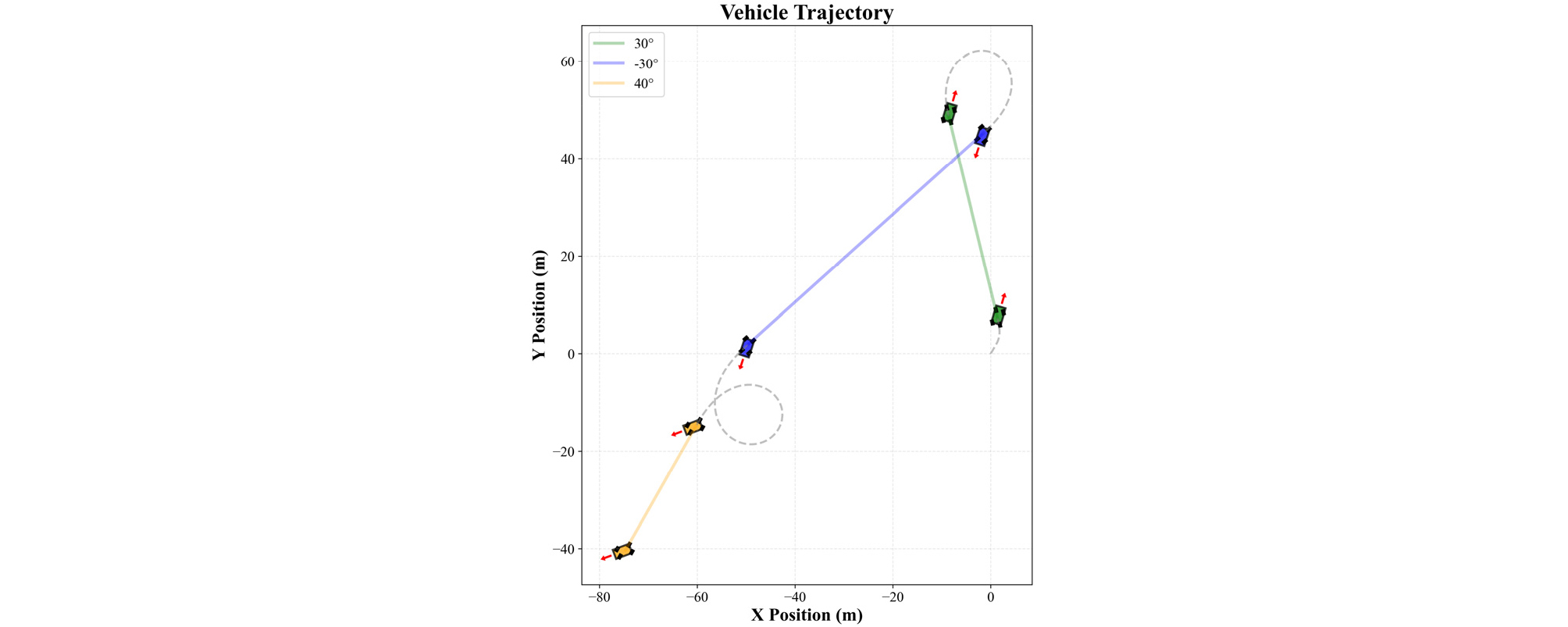
Fig. 9 presents the vehicle trajectory for this segment, where straight-line motion in an oblique direction is observed without any change in yaw. Unlike conventional driving, in which the trajectory is generated by body rotation due to steering, diagonal driving is characterized by a fixed vehicle orientation and a trajectory determined by the velocity vector direction.

Fig. 8 and Fig. 10 depict the time responses of the yaw angle and yaw rate, respectively. Throughout the diagonal driving segment, the yaw angle remains nearly constant and the yaw rate stays close to zero, indicating the absence of rotational motion and the dominance of pure translation.

These results confirm that the proposed model satisfies the kinematic definition of diagonal driving, with simultaneous longitudinal and lateral translation occurring without yaw rotation, and consistently reproduces the special motion enabled by the e-Corner vehicle architecture.

https://cdn.apub.kr/journalsite/sites/kasa/2026-018-01/N0380180107/images/kasa_18_01_07_F7.jpg

Fig. 7

Body Velocities during Diagonal Driving

https://cdn.apub.kr/journalsite/sites/kasa/2026-018-01/N0380180107/images/kasa_18_01_07_F8.jpg

Fig. 8

Yaw Angle during Diagonal Driving

https://cdn.apub.kr/journalsite/sites/kasa/2026-018-01/N0380180107/images/kasa_18_01_07_F9.jpg

Fig. 9

Vehicle Trajectory during Diagonal Driving

https://cdn.apub.kr/journalsite/sites/kasa/2026-018-01/N0380180107/images/kasa_18_01_07_F10.jpg

Fig. 10

Yaw Rate during Diagonal Driving

5. Conclusion

This study developed an integrated vehicle dynamics simulator for an e-Corner system, in which each corner independently computes driving and braking, steering, active suspension, and tire dynamics, and is coupled with a six-degree-of-freedom (6-DOF) rigid-body vehicle model. Wheel forces and states calculated at the corner level are converted into body-frame forces and moments, while body states such as roll, pitch, and vertical displacement are fed back to the corner subsystems, forming a closed-loop integrated framework.

The main contributions are as follows. First, the e-Corner vehicle was modularized into corner-based subsystems, and the signal flow and input–output relationships between the corners and the vehicle body were systematically formulated and implemented. Second, an equivalent anti-roll mechanism based on the passive stabilizer principle was realized using active suspension to physically model left–right suspension coupling. Third, comparisons with CarMaker simulation data confirmed that longitudinal and lateral motions, as well as roll and pitch responses, were well reproduced, and that translational motion without body rotation was achieved in e-Corner-specific driving modes.

Future work will focus on improving nonlinear behavior reproduction by incorporating data-driven modeling of suspension friction and backlash, actuator nonlinearities and delays, and tire nonlinear characteristics based on real vehicle data. In addition, control allocation for over-actuated e-Corner vehicles will be investigated to distribute desired body forces and moments to each corner while respecting actuator limits and tire-friction constraints. The integrated simulator will also be extended toward motion and stability control studies, including body-attitude stabilization, yaw stabilization, and trajectory tracking, to support broader vehicle motion control and autonomous driving applications.

Acknowledgements

This research was supported by the Regional Innovation System & Education (RISE) program through the (Chungbuk Regional Innovation System & Education Center), funded by the Ministry of Education (MOE) and the (Chungcheongbuk-do), Republic of Korea. (2025-RISE-11-014-03)

References

Merritt, H. E., 1967, Hydraulic Control Systems, Wiley, New York, pp. 45~62.

Limpert, R., 2011, Brake Design and Safety, SAE International, Warrendale, pp. 120~138.

10.4271/R-398

Gillespie, T. D., 1992, Fundamentals of Vehicle Dynamics, SAE International, Warrendale, pp. 65~92.

10.4271/R-114

Rajamani, R., 2012, Vehicle Dynamics and Control, 2nd ed., Springer, New York, pp. 161~185.

10.1007/978-1-4614-1433-9

Genta, G., 1997, Motor Vehicle Dynamics: Modeling and Simulation, World Scientific, Singapore, pp. 345~370.

10.1142/3329

Rajamani, R., 2012, Vehicle Dynamics and Control, 2nd ed., Springer, New York, pp. 285~320.

10.1007/978-1-4614-1433-9

Pacejka, H. B., 2012, Tire and Vehicle Dynamics, 3rd ed., Butterworth-Heinemann, Oxford, pp. 123~160.

D. J. Gillespie, 1992, Fundamentals of Vehicle Dynamics, SAE International, Warrendale, PA, pp. 205~245.

10.4271/R-114

H. B. Pacejka, 2012, Tire and Vehicle Dynamics, 3rd ed., Butterworth-Heinemann, Oxford, UK, pp. 35~52.

R. Isermann, 2014, Mechatronic Systems, Springer, Berlin, Germany, pp. 411~430.

Rajamani, R., 2006, Vehicle Dynamics and Control. Springer, USA. p. 420 pp. 348~364.

Pacejka, H. B., 2006, Tyre and Vehicle Dynamics (2nd ed.), Elsevier, Oxford, pp. 1~50.

10.1016/B978-075066918-4/50001-0

Gillespie, T. D., 1992, Fundamentals of Vehicle Dynamics. SAE International, USA. pp. 348~364.

10.4271/R-114

Gillespie, T. D., Fundamentals of Vehicle Dynamics, SAE International, Warrendale, PA, 1992, pp. 19~22.

10.4271/R-114

Ahmed A. Shabana, Dynamics of Multibody Systems, 5th ed. (Cambridge University Press, 2020), Sec. 3.11 “Newton–Euler Equations,” p. 144.

Journal of Auto-vehicle Safety Association ISSN:2005-9396(Print) 자동차안전학회지

Preview

Integrated 6-DOF Vehicle Dynamics Modeling and Simulation-Based Validation for 4-Corner Independent Driving Platforms

ABSTRACT

MAIN

Fig. 1

Block diagram of the integrated 6-DOF vehicle dynamics simulator with e-Corner modules

Table 1.

I/O of the subsystems

Table 2.

Key vehicle specifications used in simulations

(1)

(2)

(3)

(4)

(5)

(6)

(7)

(8)

(9)

(10)

(11)

(12)

(13)

(14)

(15)

(16)

(17)

(18)

(19)

(20)

(21)

(22)

(23)

(24)

(25)

(26)

(27)

(28)

(29)

(30)

Table 3.

Definition of the accel./decel. driving scenario

Table 4.

Definition of the active-function-applied sine sweep steering driving scenario

Fig. 2

Longitudinal acceleration under acceleration- deceleration

Fig. 3

Pitch rate under acceleration-deceleration

Fig. 4

Yaw rate response with active anti-roll control under sine sweep steering

Fig. 5

Roll rate response with active anti-roll control under sine sweep steering

Fig. 6

Roll angle response with active anti-roll control under sine sweep steering

Fig. 7

Body Velocities during Diagonal Driving

Fig. 8

Yaw Angle during Diagonal Driving

Fig. 9

Vehicle Trajectory during Diagonal Driving

Fig. 10

Yaw Rate during Diagonal Driving

Acknowledgements

References