Model-Based Yaw-Rate Tracking Control with Online Adaptation of Steering and Tire Parameters for an E-Corner-Based Four-Wheel Independent Steering Vehicle

Yun-m Sung; Jae-poong Lee; Jung-min Cho

doi:10.22680/kasa2026.18.1.110

Preview

Journal of Auto-vehicle Safety Association. 31 March 2026. 110-126
https://doi.org/10.22680/kasa2026.18.1.110

Model-Based Yaw-Rate Tracking Control with Online Adaptation of Steering and Tire Parameters for an E-Corner-Based Four-Wheel Independent Steering Vehicle

Yun-m Sung¹^*

Jae-poong Lee²^†

Jung-min Cho³

¹B.S. Student, Department of Intelligent Systems and Robotics, Chungbuk National University

²Assistant Professor, Department of Intelligent Systems and Robotics, Chungbuk National University

³Senior Research Engineer, Electrification Research Team, Seohan Innobility

^{*First Author}

^{†Corresponding Author}

ABSTRACT

This paper presents a model-based yaw-rate tracking control framework for an e-corner–based vehicle with four-wheel independent steering (4WIS). Owing to the over-actuated nature of the platform, accurate yaw-motion generation requires a consistent connection among vehicle yaw dynamics, tire lateral-force generation, and steering actuator dynamics. A hierarchical feedforward framework is developed to map a desired yaw-rate profile to the required yaw moment, allocate it to per-wheel lateral-force commands, and convert them into per-wheel steering angle and steering motor torque commands via an inverse actuator model. While feedforward control provides fast response and physical interpretability, its performance can degrade under steering actuator uncertainties, tire-parameter variations, and unmodeled disturbances.

To mitigate these effects without introducing overly complex robust-control structures, a recursive least-squares (RLS)–based parameter adaptation scheme is integrated into the feedforward pipeline. The proposed method estimates and updates the key model parameters—namely the steering actuator viscous damping and the tire cornering stiffness—from input–output data, and uses the updated parameters to align the feedforward torque/steering command generation with the actual vehicle response. The proposed approach is evaluated in simulation under a deliberate 10% mismatch in the viscous damping and cornering stiffness parameters. Comparative studies are conducted for four configurations: feedforward only, feedforward with yaw-rate feedback, feedforward with RLS adaptation, and feedforward with both RLS adaptation and feedback. The results show that RLS-based adaptation improves yaw-rate tracking robustness under parameter uncertainty and reduces reliance on feedback compensation, achieving stable tracking performance across uncertainty scenarios.

Keywords

Vehicle dynamics

e-Corner system

Yaw-rate tracking

Model-based feedforward

Recursive least squares

MAIN

1. Introduction
2. e-Corner (4WIS) Vehicle Plant Modeling
2.1. Planar Vehicle Kinematics and Corner Geometry
2.2. Tire–Steering Actuator Model
3. Yaw-Rate Tracking Controller Design
3.1. Hierarchical Control Architecture
3.2. Target Yaw-Moment Generation
3.3. Yaw-Moment to Corner Lateral-Force Allocation(F_y,i,ref)
3.4. Inverse Model from Lateral Force to Steering Angle
3.5. Steering-Torque Reference Synthesis and Steering-Angle Compensation
4. Online Estimation and Compensation of Steering and Tire Parameters
4.1. Necessity of Online Adaptation under Parameter Mismatch
4.2. Adaptive Parameter Estimation (Regression + Update)
4.3. Integration into the Controller
5. Simulation-Based Performance Evaluation and Analysis
5.1. Simulation Setup and Scenario Design
5.2. Compared Cases and Evaluation Metrics
5.3. Scenario-Wise Yaw-Rate Tracking Results
5.4. Diagnosis of Online Adaptation Performance Degradation
6. Conclusion

1. Introduction

With the advancement of electrified chassis technologies, corner-module–based platforms that integrate driving, steering, and braking functions at the wheel level have attracted significant attention as a promising form of next-generation mobility. In particular, e-corner–based vehicles provide independent driving/steering/braking degrees of freedom for each wheel, thereby forming an over-actuated system capable of generating diverse combinations of forces and moments even under identical driving conditions. Although this architecture offers clear advantages in maneuverability and chassis-control performance, it inevitably involves the problem of generating and distributing control inputs to achieve a desired vehicle motion, including control allocation and lower-level actuator control.

This study focuses on yaw-rate ( $r$ ) tracking for a 4WIS e-corner vehicle. In a 4WIS configuration, yaw dynamics are primarily governed by tire lateral forces generated through wheel steering; therefore, fast and accurate yaw-rate tracking requires a model-based control structure that consistently connects the vehicle dynamics, tire lateral-force generation, and steering actuator dynamics. Model-based feedforward (FF) control provides high responsiveness and physical interpretability by computing the required yaw moment ( $M_{z}$ ) from the desired yaw-rate command and converting it into per-wheel lateral-force and steering inputs. However, in practical systems, model mismatch may arise due to variations in the steering actuator viscous parameter $B$ , nonlinear friction/disturbances, and changes in tire–road conditions that affect the cornering stiffness ( $c_{α}$ ). Under such mismatches, the steering angle and torque commands produced by the feedforward pipeline may become inconsistent with the actual lateral-force generation, resulting in degraded tracking performance. Hence, it is necessary to design a controller that preserves the model-based framework while incorporating a compensation mechanism to align the model with actuator and tire uncertainties.

To this end, this paper proposes a hierarchical feedforward control framework based on an integrated e-corner vehicle model, consisting of the following stages: required yaw-moment generation, per-wheel lateral-force allocation, per-wheel steering-angle computation, and steering torque calculation using an inverse steering actuator model. To compensate for residual tracking errors caused by model mismatch, a feedback (FB) controller (PID) is additionally combined with the feedforward structure. Furthermore, to suppress performance degradation under parameter uncertainties of up to ±10% in the steering viscous damping $B$ and the tire cornering stiffness $c_{α}$ , a recursive least squares (RLS)–based parameter adaptation scheme is introduced. The proposed method estimates and updates $B$ and $c_{α}$ online from measured input–output data during driving, and reflects the updated parameters in the feedforward torque/steering command generation, thereby improving the consistency between the model-based commands and the actual vehicle response. This approach enhances yaw-rate tracking performance by restoring the accuracy of model-based feedforward control without resorting to excessively complex robust-control structures.

2. e-Corner (4WIS) Vehicle Plant Modeling

This section summarizes the plant model of an e-corner–based 4WIS vehicle. The plant model describes how each wheel’s steering input and lateral force contribute to the vehicle yaw-rate response, and it serves as the basis of the model-based feedforward control chain used in Section 3.

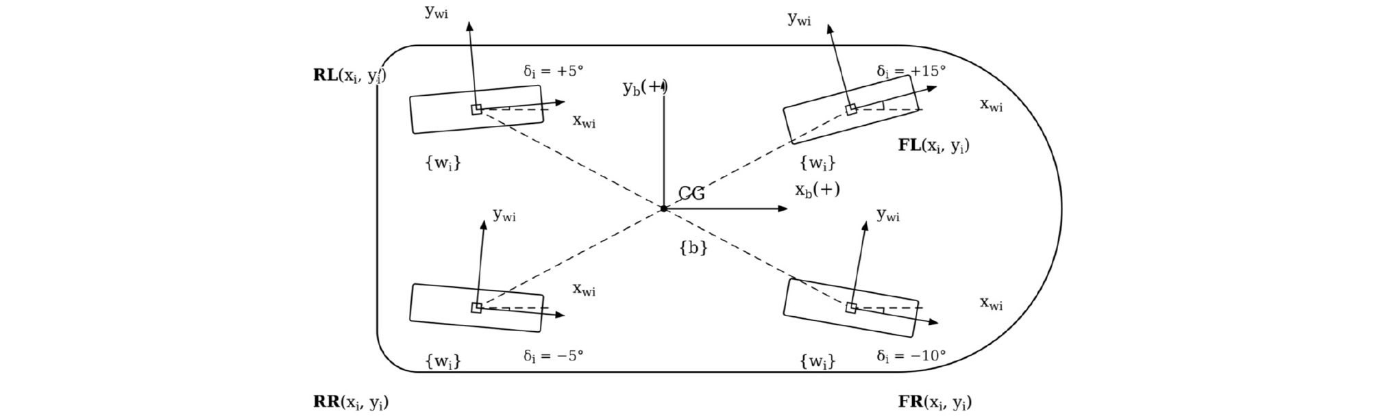
2.1. Planar Vehicle Kinematics and Corner Geometry

The vehicle is described using a body-fixed coordinate frame $\{b\}$ centered at the center of gravity (CG), where the x-axis points forward (+), the y-axis points to the left (+), and the z-axis points upward (+). The yaw-rate is defined positive in the counterclockwise (CCW) direction about the +z axis. Each corner (wheel) is indexed as $i \in \{F L, F R, R L, R R\}$ , and the corner location with respect to the CG is denoted by $(x_{i}, y_{i})$ . The steering angle at each corner is $δ_{i}$ , and when $δ_{i} = 0$ , the wheel heading is aligned with the body x-axis.

https://cdn.apub.kr/journalsite/sites/kasa/2026-018-01/N0380180109/images/kasa_18_01_09_F1.jpg

Fig. 1

Plan-view schematic of the vehicle and the body/wheel coordinate frames

The planar motion state of the vehicle is represented by $(V_{x}, V_{y}, r)$ . The velocity of each corner expressed in the body frame is computed from rigid-body kinematics as

(1)

V_{x, i}^{b} = V_{x} - r y_{i} V_{y, i}^{b} = V_{y} - r x_{i}

2.2. Tire–Steering Actuator Model

In this section, we summarize the coupled structure in which the steering actuator at each corner generates the steering angle $δ_{i}$ . The slip angle (slip angle, $α_{i}$ ) is determined by the steering angle and the corner velocity, and then the tire lateral force $F_{y, i}$ and the self-aligning torque (aligning torque, $T_{a l i g n, i}$ ) are generated and fed back as a reaction torque to the steering axis.

2.2.1. Wheel Coordinate Frame Definition and Velocity Transformation

For corner $i$ , the wheel coordinate frame $\{w_{i}\}$ is defined as the body coordinate frame $\{b\}$ rotated by the steering angle $δ_{i}$ . The corner velocity expressed in the body frame $(V x_{i}^{b}, V y_{i}^{b})$ is transformed into the wheel frame $\{w_{i}\}$ as follows:

(2)

[\begin{matrix} [V_{x, i}^{w}] \\ [V_{y, i}^{w}] \end{matrix}] = R (- δ_{i}) [\begin{matrix} [V_{x, i}^{b}] \\ [V_{y, i}^{b}] \end{matrix}]

2.2.2. Slip Angle( $α_{i}$ ) and Tire Lateral-Force Model

The slip angle is defined based on the wheel-frame velocity:

(3)

α_{i} = \tan^{- 1} \frac{V_{y, i}^{w}}{V_{x, i}^{w}}

The tire lateral force is modeled using a linear cornering stiffness $c_{α}$ ,

(4)

F_{y, i}^{w} = - C_{α} α_{i}

To account for the friction limit, a saturation constraint is applied:

(5)

|F_{y, i}^{w}| \leq μ F_{z, i}

where $μ$ is the friction coefficient and $F z_{i}$ is the vertical load at corner $i$ .

2.2.3. Self-Aligning Torque( $T_{a l i g n}$ )

The aligning torque is modeled using a trail-based approximation:

(6)

T_{a l i g n, i} \approx t r a i l_{i} \cdot F_{y, i}^{w}

This torque acts as a restoring component that tends to return the steering angle in the direction that reduces the slip angle. As a result, it is coupled into the steering actuator dynamics as a disturbance (reaction torque). In implementation, the sign convention is selected consistently so that $T_{a l i g n, i}$ becomes a restoring torque according to the positive-direction definitions of $δ_{i}$ and $F_{y, i}^{w}$ .

2.2.4. Steering Actuator Dynamics (Plant)

The steering axis of each corner is approximated by a second-order model using an equivalent inertia and viscous damping:

(7)

J_{δ} {\ddot{δ}}_{i} + B_{δ} {\dot{δ}}_{i} = N_{g} T_{s t r, i} - T_{a l i g n, i}

Here, $J_{δ}$ is the equivalent steering-axis inertia, $B_{δ}$ is the viscous damping coefficient, $T_{s t r, i}$ is the steering motor input torque, and $N_{g}$ is the gear ratio between the motor and the steering axis. The parameters $J_{δ}$ , $B_{δ}$ and $C_{α}$ may involve uncertainties due to environmental conditions, temperature, wear, and modeling errors. The influence of uncertainties in $B_{δ}$ and $C_{α}$ , as well as the correction method, will be discussed in the subsequent sections.

2.2.5. Corner-Force Transformation to the Body Frame and Yaw-Moment Synthesis

Since the tire forces are computed in the wheel coordinate frame, they are transformed into the body coordinate frame. The force transformation is given by

(8)

[\begin{matrix} F_{x, i}^{b} \\ F_{y, i}^{b} \end{matrix}] = R (δ_{i}) \cdot [\begin{matrix} F_{x, i}^{w} \\ F_{y, i}^{w} \end{matrix}]

The vehicle yaw moment $M_{z}$ is synthesized from the corner forces as

(9)

M_{z} = \sum_{i} (x_{i} F_{y, i}^{b} - y_{i} F_{x, i}^{b})

Finally, the yaw dynamics are represented as

(10)

I_{z z} \cdot \dot{r} = M_{z}

where $I_{z z}$ is the yaw moment of inertia. Since this paper focuses on yaw-rate tracking, the subsequent controller design generates the target yaw moment based on Eq. (9)–(10) and distributes it into corner forces.

3. Yaw-Rate Tracking Controller Design

This section designs a yaw-rate tracking controller based on the plant model formulated in Section 2. Since a 4WIS vehicle has independent steering inputs at each corner, it is natural to decompose the yaw-rate tracking problem into the following stages: yaw-moment generation, corner-force allocation, steering-angle generation, and steering-torque generation. As shown in Fig. 2, this study adopts a hierarchical control architecture, where the subscript “ref” denotes reference signals generated by the controller.

https://cdn.apub.kr/journalsite/sites/kasa/2026-018-01/N0380180109/images/kasa_18_01_09_F2.jpg

Fig. 2

Block diagram of the proposed hierarchical yaw-rate tracking control architecture

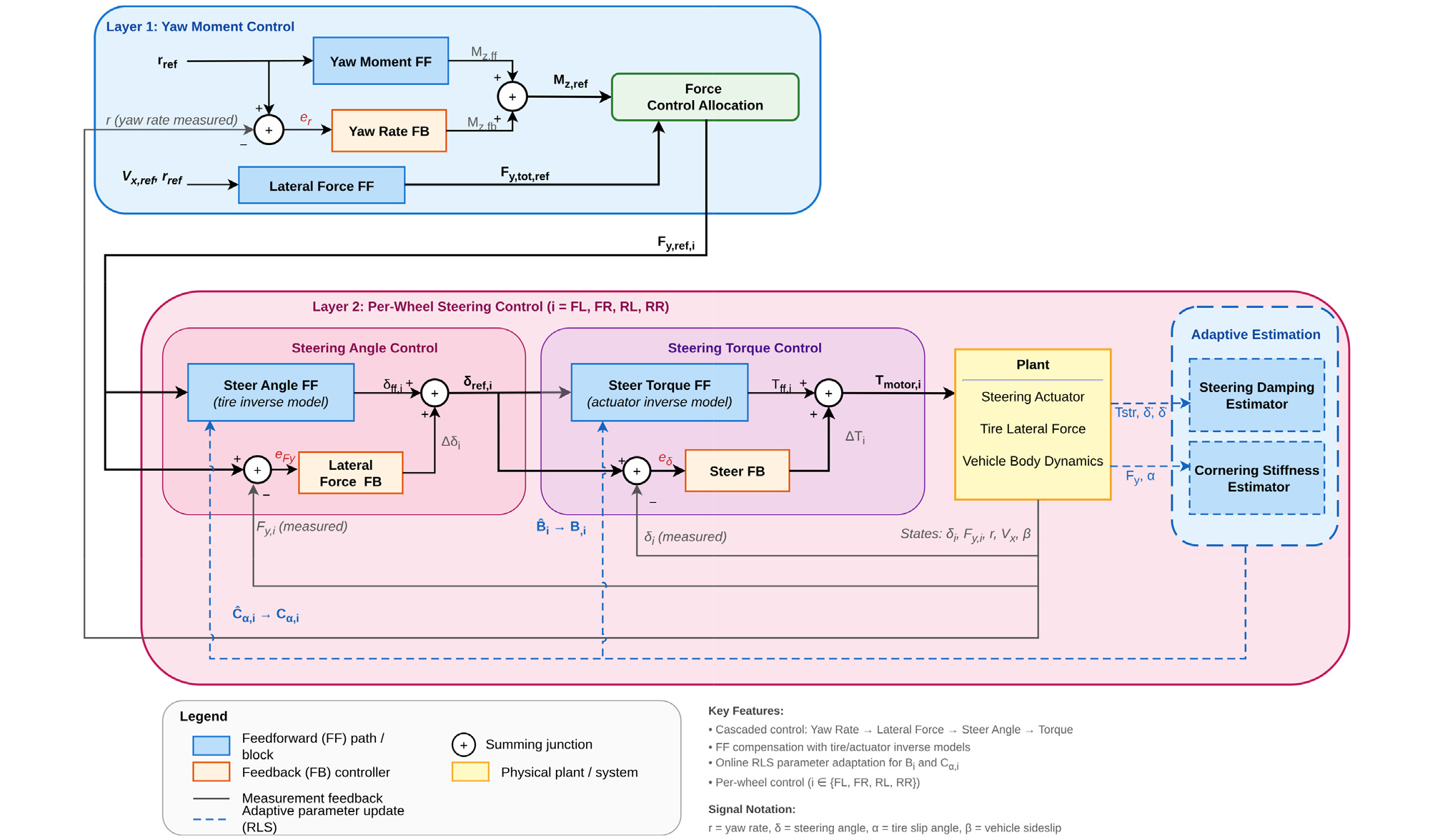
3.1. Hierarchical Control Architecture

As illustrated in Fig. 2, the controller first computes the target yaw moment $M_{z, r e f}$ from the yaw-rate error. Then, the desired yaw moment is allocated into corner lateral-force references $F_{y, i, r e f}$ . Using an inverse tire model, $F_{y, i, r e f}$ is converted into steering-angle references $δ_{i, r e f}$ , and finally, the steering actuator model is used to generate the steering torque reference $T_{s t r, i, r e f}$ for tracking $δ_{i, r e f}$ . Since each stage employs intermediate variables with clear physical meaning, the proposed structure is convenient for analyzing and comparing control performance in over-actuated systems.

3.2. Target Yaw-Moment Generation

The yaw-rate error is defined as

(11)

e_{r} = r_{r e f} - r

The target yaw moment is composed of a feedforward term and a feedback term:

(12)

M_{z, r e f} = M_{z, f f} + M_{z, f b}

The feedforward yaw moment is determined from the yaw dynamics (10) as

(13)

M_{z, f f} = I_{z z} \cdot {\dot{r}}_{r e f}

The feedback term is configured in a PID (or PD) form based on $e_{r}$ .

(14)

M_{z, f b} = K_{p, r} e_{r} + K_{i, r} \int e_{r} d t + K_{d, r} {\dot{e}}_{r}

3.3. Yaw-Moment to Corner Lateral-Force Allocation(F_y,i,ref)

In this paper, the control allocation problem is not formulated as an optimization problem. Instead, the yaw-moment component and the total lateral-force component are uniformly distributed among the four corners to construct the reference lateral forces. First, the target yaw moment is equally shared:

(15)

M_{z, i, r e f} = \frac{1}{4} M_{z, r e f}

In addition, the required total lateral-force level for the target yaw dynamics is approximated as

(16)

F_{y, t o t a l, r e f} \approx m V_{x, r e f} r_{r e f}

By equally distributing this term and combining it with the yaw-moment–induced lateral-force component, the final corner lateral-force reference is constructed as

(17)

F_{y, i, r e f} = F_{y, i, r e f}^{(M)} + \frac{1}{4} F_{y, t o t a l, r e f}

where $F_{y, i, r e f}^{(M)}$ denotes the lateral force required at each wheel to generate $M_{z, r e f}$ .

3.4. Inverse Model from Lateral Force to Steering Angle

This subsection generates the reference steering angle that satisfies the desired corner lateral force. The tire model follows Eq. (4)–(5). In the linear region, the inverse of Eq. (4) yields

(18)

α_{i, r e f} = - \frac{F_{y, i, r e f}}{C_{α, i}}

The velocity direction angle at the corner is computed from the kinematics (1) and the velocity transformation (2), and is denoted as $β_{i, r e f}$ . Using the slip-angle relation

(19)

α_{i} = β_{i} - δ_{i}

the steering-angle reference is obtained as

(20)

δ_{i, r e f} = β_{i, r e f} - α_{i, r e f}

3.5. Steering-Torque Reference Synthesis and Steering-Angle Compensation

The steering drive unit generates a motor torque reference to track $δ_{i, r e f}$ . This study constructs a feedforward steering torque based on the equivalent steering-axis model and optionally adds a PID correction torque based on the steering-angle error. The steering-angle error is defined as

(21)

e_{δ, i} (t) = δ_{i, r e f} (t) - δ_{i} (t)

and the final torque reference is given by

(22)

T_{s t r, i, r e f} (t) = T_{s t r, i, f f} (t) + T_{s t r, i, f b} (t)

Here, $T_{s t r, i, f f}$ includes the velocity/acceleration terms of $δ_{i, r e f}$ as well as the aligning-torque compensation term, whereas $T_{s t r, i, f b}$ compensates $e_{δ, i}$ using a PID form.

4. Online Estimation and Compensation of Steering and Tire Parameters

In this chapter, an adaptive parameter compensator is formulated to estimate the steering damping coefficient $B_{δ}$ and the tire cornering stiffness $C_{α}$ online, considering that uncertainties in these two parameters can deteriorate the consistency between steering angle and lateral force. The proposed compensator is based on linear regression models derived from the steering dynamics and the linear tire lateral force model, and the estimated parameters are directly substituted into the corresponding model parameters inside the controller. In this study, the equivalent steering inertia $J_{δ}$ is treated as a nominal constant, and the scope of online compensation is limited to $B_{δ}$ and $C_{α}$ .

4.1. Necessity of Online Adaptation under Parameter Mismatch

The coupled steering–tire model used in this study can describe yaw-rate behavior with a limited set of parameters; however, if the parameters deviate from their nominal values, the consistency of model-based terms may degrade. The damping coefficient $B_{δ}$ directly affects the dynamic characteristics (gain and phase) of the steering-angle response, while the cornering stiffness $C_{α}$ determines the scale of the slip-angle–lateral-force relationship. Therefore, mismatches in these parameters appear as steering-angle tracking errors or lateral-force reproduction errors, which eventually lead to degraded yaw-rate tracking performance. To mitigate such effects, this chapter estimates $B_{δ}$ and $C_{α}$ online and reflects them in the controller.

The estimation is constructed in a linear regression form using signals available from simulation. Specifically, $B_{δ}$ is estimated by treating the inertia term of the steering-axis dynamics as a nominal value $J_{δ, n o m}$ and expressing the residual term as a linear relationship with the steering-angle rate. Meanwhile, $C_{α}$ is estimated using the linear relationship between the lateral force $F_{y}$ and slip angle $α$ in the linear tire model.

For each corner $i$ , the estimates are denoted as ${\hat{B}}_{δ, i}$ and ${\hat{C}}_{α, i}$ , which are updated by the parameter update law in the next section and applied in a plug-in manner while keeping the controller structure unchanged.

4.2. Adaptive Parameter Estimation (Regression + Update)

This section constructs a recursive least squares (RLS)-based online estimator for the two parameters $B_{δ}$ and $C_{α}$ defined in Section 4.1. The estimator operates in discrete time and introduces a forgetting factor $λ$ to track time-varying parameters. In addition, to prevent performance degradation caused by data collected in constrained regions or outside the valid model range, the update is performed only over conditionally selected time intervals. The following subsections describe the update rule, the data construction for estimating $B_{δ}$ , and the data construction and update-window criteria for estimating $C_{α}$ .

4.2.1. Scalar Parameter Update

For computational efficiency and implementation simplicity, each parameter is estimated as a scalar. Assuming a linear relationship between the observation $y (k)$ and the regressor $ϕ (k)$ for parameter $θ$ , the regression model is given by

(23)

y (k) = θ ϕ (k) + ε (k)

Using the forgetting factor $λ, (0 < λ \leq 1)$ , the scalar update rule computes the gain $K (k)$ based on the previous estimate $\hat{θ} (k - 1)$ and updates $\hat{θ} (k)$ proportionally to the estimation error. The covariance $P (k)$ is updated using the same forgetting factor, which enables tracking of time variations by assigning higher weights to recent data. The initial conditions are set as

(24)

\hat{θ} (0) = θ_{0}, P (0) = p_{0}

For numerical stability, the update is skipped if the denominator becomes abnormal, and the estimate is bounded by upper and lower limits to remain physically plausible. These constraints aim to mitigate divergence due to outliers or model mismatch that can occur during online estimation.

4.2.2. Estimation of Steering Damping Coefficient $B_{δ}$

In the steering-axis dynamics, the damping coefficient appears as a linear term with respect to the steering-angle rate. In this study, the equivalent steering inertia $J_{δ}$ is treated as a nominal value, and, $B_{δ}$ is estimated by constructing the observation as the residual torque after removing the inertia term. Specifically, the net torque is computed from the driving torque applied to the steering axis and the reaction torque from the tire, and then the inertia term is compensated so that the component corresponding to the damping term is used for estimation. The regressor is set as the steering-angle rate ${\dot{δ}}_{i}$ , and $B_{δ, i}$ is updated from the proportional relationship between the inertia-compensated net torque and ${\dot{δ}}_{i}$ .

However, when the steering-angle rate is sufficiently small, the signal-to-noise ratio decreases and the estimation may become unstable. Moreover, near the steering-angle limit or the steering-rate limit, the plant behavior is dominated by the constraints, reducing the validity of the regression model. Therefore, the update of $B_{δ}$ is performed only when ${\dot{δ}}_{i}$ exceeds a certain threshold, the steering angle is sufficiently away from mechanical limits, and the steering rate has enough margin from the maximum rate limit. Samples that yield invalid computed signals are also excluded. This conditional update selection is designed to ensure stable convergence even under the parameter randomization conditions presented in Chapter 5.

4.2.3. Estimation of Cornering Stiffness $C_{α}$

In the linear region of the tire lateral force model, the lateral force is proportional to the slip angle; hence, $C_{α}$ can be estimated from the linear relationship between $F_{y, i}$ and $α_{i}$ . In this study, $α_{i}$ is used as the regressor and $F_{y, i}$ as the observation to update $C_{α, i}$ online.

When the lateral force saturates due to the friction limit, the linear proportional relationship no longer holds; thus, time intervals close to saturation are excluded from the update. In particular, if $F_{y, i}$ exceeds a certain ratio relative to the limit defined by the vertical load $F_{z, i}$ and friction coefficient $μ_{i}$ , the update is not performed. Additionally, if $α_{i}$ is excessively small, numerical instability may occur; therefore, only samples with $|α_{i}|$ greater than a predefined threshold are used.

In summary, the $C_{α}$ estimator selects update intervals such that only data within the valid linear-tire region are used, ensuring that the estimate reflects the “effective cornering stiffness in the linear region.” Chapter 5 presents both the convergence characteristics under different saturation-margin and slip-angle thresholds and the resulting yaw-rate tracking performance changes.

4.3. Integration into the Controller

The corner-wise estimates ${\hat{B}}_{δ, i}$ , ${\hat{C}}_{α, i}$ obtained in Section 4.2 are incorporated without changing the controller structure, by directly substituting the corresponding parameters included in the model-based terms. That is, the signal flow and feedback gains defined in Chapter 3 remain unchanged, while the estimates are applied only at the following two locations.

First, the cornering stiffness used for computing the slip-angle reference in the lateral-force inverse model is replaced by ${\hat{C}}_{α, i}$ instead of the nominal value. This reduces the scale mismatch between the target lateral force and the target slip angle (and steering angle).

Second, the coefficient used in the damping term of the steering torque feedforward is replaced by ${\hat{B}}_{δ, i}$ instead of the nominal value. The equivalent steering inertia $J_{δ}$ is maintained as a nominal value, and the scope of online compensation is limited to the damping coefficient and cornering stiffness.

The estimates are updated in discrete time, and the updated values are reflected in the computation of the next step. Furthermore, before sufficient data have been accumulated to form reliable estimates, the nominal values are retained, and ${\hat{B}}_{δ, i}$ and ${\hat{C}}_{α, i}$ are applied only after a minimum number of samples. The update-window selection and estimate bounding follow the criteria defined in Section 4.2.

Remark on closed-loop stability: Since the proposed framework updates only the feedforward model parameters ( ${\hat{B}}_{δ, i}$ , ${\hat{C}}_{α, i}$ ) while keeping the controller structure and feedback gains unchanged, the nominal closed-loop stability ensured by the feedback loop is preserved. The online adaptation therefore acts as a bounded, slowly varying modification of the feedforward terms. To avoid destabilizing transients, parameter updates are activated only after a minimum number of valid samples are accumulated, abnormal updates are skipped, and all estimates are bounded to remain physically plausible. Under these safeguards, the overall system can be regarded as a bounded time-varying system with maintained closed-loop stability.

5. Simulation-Based Performance Evaluation and Analysis

5.1. Simulation Setup and Scenario Design

This section evaluates the proposed yaw-rate tracking control architecture through simulation and analyzes the contribution of online parameter adaptation under uncertainty. The common simulation settings—time step $∆ t$ , total duration $T$ , and target longitudinal speed $v_{x}$ —are summarized in Table 1. The desired yaw-rate reference is defined as a sine wave, and its parameters (amplitude $A_{r}$ , frequency $f$ , start delay $t_{d}$ , and ramp time $t_{r}$ ) as well as the uncertainty conditions vary depending on the scenario, as listed in Table 2.

Table 1.

Simulation settings

Item		Symbol	Value	Notes
Time step		$∆ t$	0.001	s
Simulation duration		$T$	30.0	s
Target speed		$v_{x}$	10.0	m/s
Target yaw-rate (Sine)	Amplitude	$A_{r}$	Table 2	rad/s
	Frequency	$f$		Hz
	Start delay	$t_{d}$		s
	Ramp time	$t_{r}$		s
Uncertainty type		-		-

Table 2.

Simulation settings

Scenario	$A_{r}$ (rad/s)	$f$ (Hz)	$t_{d}$ (s)	$t_{r}$ (s)	Uncertainty
1	0.30	0.50	1.0	2.0	static (±10% bias)
2	0.30	0.50	1.0	2.0	dynamic (random)
3	0.50	0.10	1.0	30.0	dynamic (random)

Three scenarios are considered. Scenario 1 imposes a fixed static bias of ±10% on the steering and tire parameters, serving as a baseline case to characterize residual errors under constant model mismatch. Scenario 2 introduces time-varying parameter perturbations (dynamic mismatch) to assess the effectiveness of online adaptation in the presence of temporal uncertainty. Scenario 3 maintains the dynamic mismatch setting but employs a more gradual excitation (including a long ramp-up), enabling additional analysis of long-term mean errors and drift components.

All comparisons are conducted using the same controller structure and identical gain settings, ensuring that performance differences originate from the inclusion of online adaptation rather than any structural modifications. In this framework, online adaptation improves internal consistency by updating the effective parameters used in reference generation (yaw moment–lateral force–steering relationship), thereby reducing mismatch-induced discrepancies.

5.2. Compared Cases and Evaluation Metrics

To isolate the contribution of online parameter adaptation (OPA), four controller configurations are evaluated under the same plant and simulation settings. The compared cases include a model-based feedforward controller (FF), a feedforward controller augmented with yaw-rate error feedback compensation (FF+FB), a feedforward controller equipped with online parameter adaptation (FF+OPA), and the combined structure that incorporates both feedback and online adaptation (FF+FB+OPA). Here, OPA denotes the online parameter update module embedded in the controller, which updates the effective steering and tire parameters used in the reference-generation pipeline.

Tracking performance is primarily assessed using the yaw-rate error, while quantitative indices include the root mean square error (RMSE) and the peak absolute error. In addition, to examine the internal consistency of the model-based control chain, auxiliary error measures are computed for the yaw moment, a representative corner lateral force, and the steering angle. RMSE results are summarized in Table 3, peak error results are provided in Table 4, and representative time-domain responses are illustrated in Fig. 3–Fig. 5.

Table 3.

RMSE comparison of yaw-rate tracking controllers

Controller	$e_{r}$ [rad/s]	$e_{M z}$ [N·m]	$e_{F y}$ [N]	$e_{δ}$ [rad]
Scenario1
FF	0.00513	46.88	21.63	0.00273
FF+FB	0.00450	41.60	17.18	0.00211
FF+OPA	0.00898	24.72	30.09	0.04377
FF+FB+OPA	0.00246	21.66	9.84	0.00151
Scenario2
FF	0.01820	35.52	59.766	0.11688
FF+FB	0.00458	36.10	25.930	0.00287
FF+OPA	0.03139	46.32	110.131	0.17556
FF+FB+OPA	0.00389	25.41	20.977	0.00312
Scenario3
FF	0.007775	8.374	18.633	0.00937
FF+FB	0.003071	6.772	17.475	0.00231
FF+OPA	0.002626	6.043	8.629	0.00551
FF+FB+OPA	0.001875	5.874	8.450	0.00099

Table 4.

Peak error comparison of yaw-rate tracking controllers

Controller	$\|e_{r}\|$ [rad/s]	$\|e_{M z}\|$ [N·m]	$\|e_{F y}\|$ [N]	$\|e_{δ}\|$ [rad]
Scenario1
FF	0.00792	68.49	33.34	0.00628
FF+FB	0.00693	65.93	28.03	0.00334
FF+OPA	0.02131	43.7	123.17	0.12201
FF+FB+OPA	0.00693	44.5	33.529	0.00334
Scenario2
FF	0.0346	147.2	192.65	0.28504
FF+FB	0.0139	145.3	90.19	0.00895
FF+OPA	0.0812	233.6	427.8	0.46921
FF+FB+OPA	0.0117	116.2	91.30	0.00939
Scenario3
FF	0.02440	52.18	152.96	0.04694
FF+FB	0.00720	35.04	106.49	0.00727
FF+OPA	0.00900	39.38	111.56	0.01455
FF+FB+OPA	0.00710	38.52	112.86	0.00373

https://cdn.apub.kr/journalsite/sites/kasa/2026-018-01/N0380180109/images/kasa_18_01_09_F3.jpg

Fig. 3

Scenario 1: Static parameter uncertainty

https://cdn.apub.kr/journalsite/sites/kasa/2026-018-01/N0380180109/images/kasa_18_01_09_F4.jpg

Fig. 4

Scenario 2: Dynamic parameter uncertainty

https://cdn.apub.kr/journalsite/sites/kasa/2026-018-01/N0380180109/images/kasa_18_01_09_F5.jpg

Fig. 5

Scenario 3: Dynamic parameter uncertainty with long ramp-up (gradual excitation)

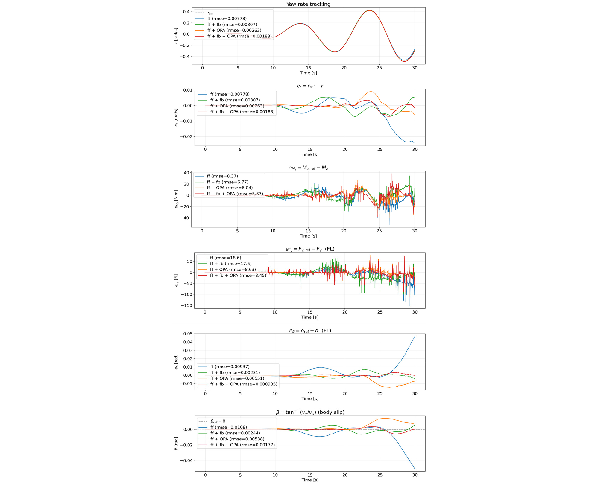
5.3. Scenario-Wise Yaw-Rate Tracking Results

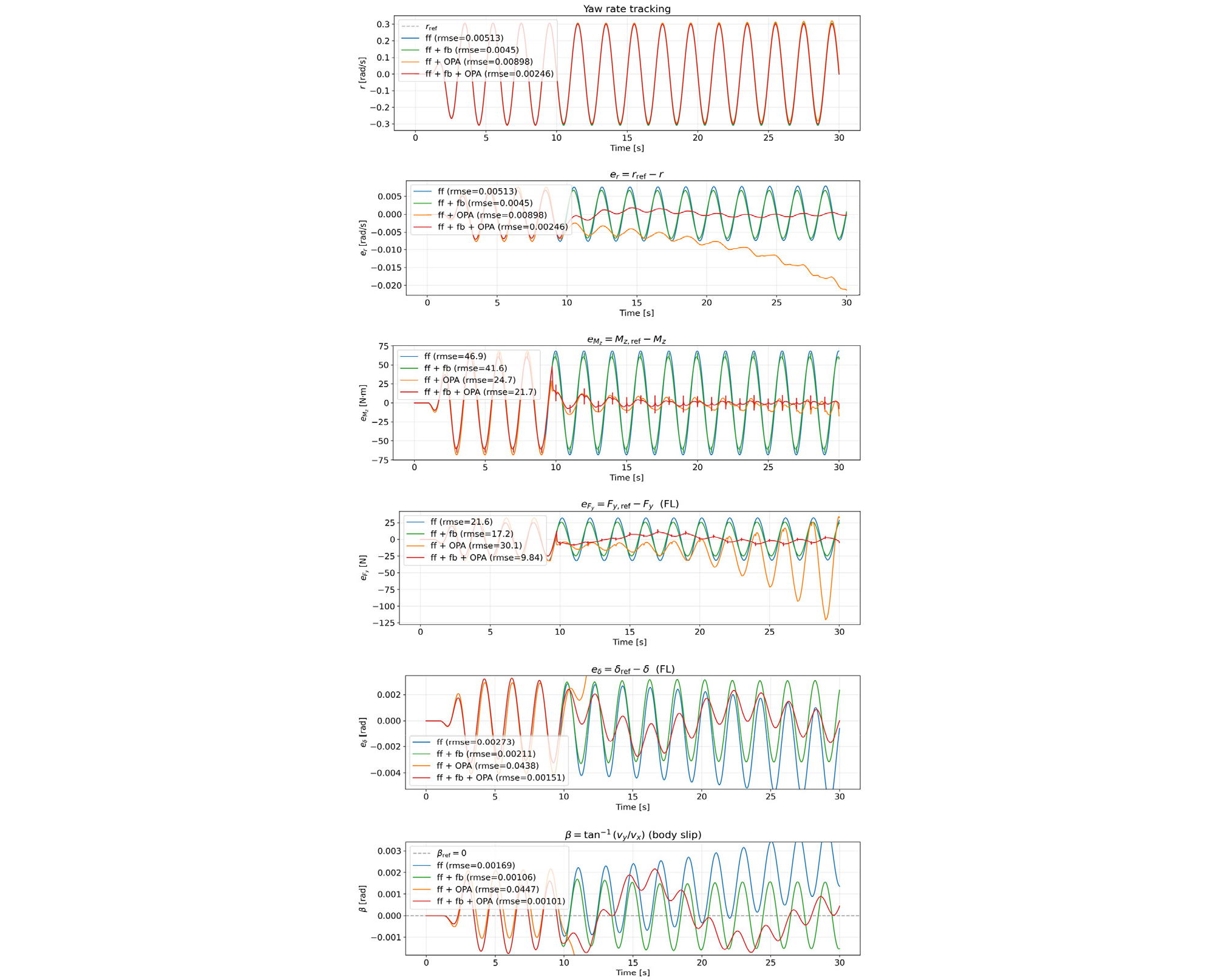
Fig. 3–Fig. 5 present the time histories of major error signals under the three scenarios defined in Table 2. Overall, the FF+FB+OPA configuration consistently maintains the smallest error levels and exhibits stable yaw-rate tracking behavior across scenarios. This trend indicates that feedback compensation effectively suppresses residual tracking errors, while online adaptation improves the consistency of the model-based reference generation by mitigating the impact of parameter mismatch.

In Scenario 1 (static mismatch), a fixed parameter bias produces a persistent offset in the model-based reference generation, which appears as a sustained error component in yaw-rate tracking. When online adaptation is included, the mean component of the yaw-rate error is reduced, and the RMSE tends to improve accordingly. However, peak errors are often dominated by transient phases, which can limit the extent of peak-error reduction even when the steady mismatch is compensated. Moreover, cases without feedback may exhibit accumulation of internal errors, further highlighting the stabilizing role of feedback in maintaining robust tracking under biased conditions.

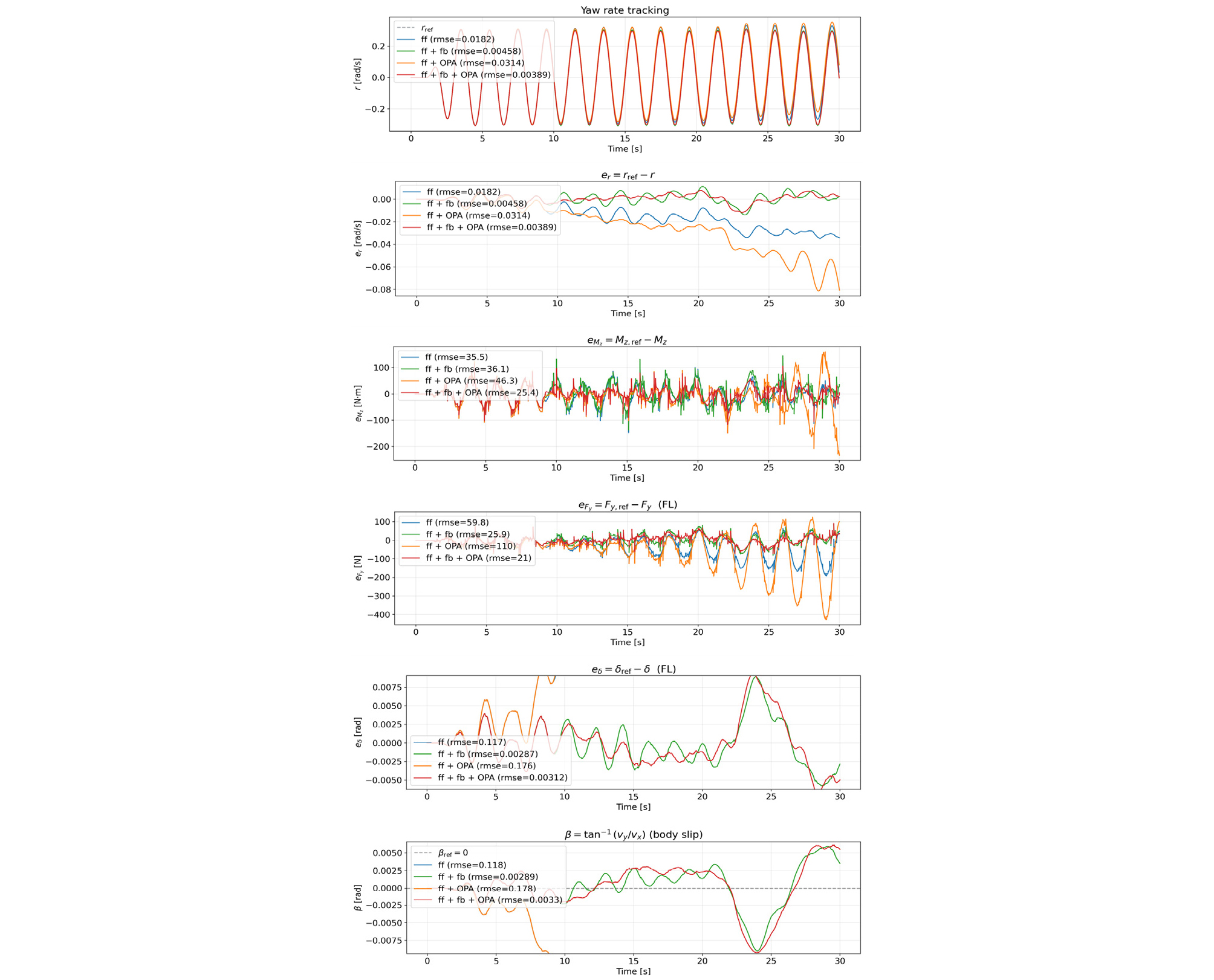
In Scenario 2 (dynamic mismatch), time-varying uncertainties can cause mismatch-induced errors to accumulate when the controller relies on fixed nominal parameters. Under this setting, online adaptation generally improves yaw-rate tracking and also reduces internal inconsistency errors associated with yaw moment generation and the lateral force–steering relationship. This observation suggests that updating the effective steering and tire parameters online helps preserve the alignment between the model-based command generation and the actual vehicle response under temporal variations. Nevertheless, when online adaptation is applied without feedback (FF+OPA), the resulting performance may be limited or may even degrade depending on the operating condition, and the underlying reasons are investigated in Section 5.4.

Scenario 3 (dynamic mismatch with long ramp-up) provides a clearer view of long-term mean errors and drift, as the excitation increases gradually over an extended interval. In this scenario, FF+FB+OPA again achieves low error levels and maintains improved consistency in the yaw moment–lateral force–steering chain over longer time scales. In contrast, configurations without feedback may suffer from unreliable parameter updates during weakly excited intervals, where informative data are insufficient for stable regression-based estimation. These results imply that online adaptation benefits from practical safeguards and is most effective when combined with feedback compensation to prevent unfavorable error accumulation and maintain stable tracking performance.

5.4. Diagnosis of Online Adaptation Performance Degradation

Under certain conditions, online adaptation may not yield the expected improvement, and in some cases the adaptation-only configuration (FF+OPA) can produce unfavorable results. This section investigates the underlying causes using diagnostic plots. Fig. 6 compares the estimated steering parameters across scenarios, together with key signals affecting regression quality, including steering angular acceleration $\ddot{δ}$ and aligning torque $T_{a l i g n}$ . Diagnostic results for Scenarios 1–3 are presented in Fig. 6 in order.

https://cdn.apub.kr/journalsite/sites/kasa/2026-018-01/N0380180109/images/kasa_18_01_09_F6.jpg

Fig. 6

Diagnostic plots for parameter adaptation (Scenario 1-3)

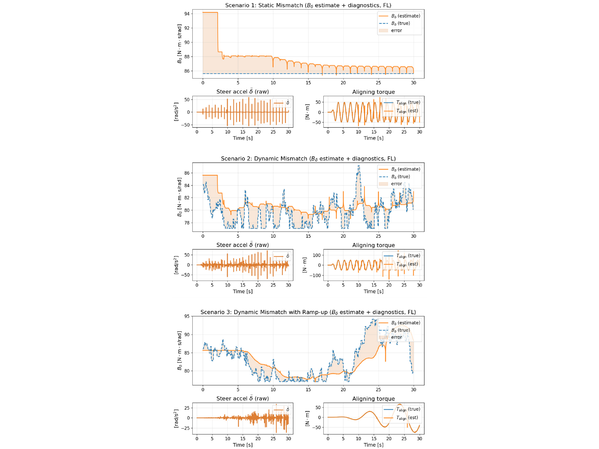
First, $\ddot{δ}$ is obtained via numerical differentiation of the steering-angle signal. Without filtering, high-frequency components can be significantly amplified, producing spike-like behavior. The step-like or abrupt changes in the parameter estimates observed in such intervals suggest that differentiation noise can corrupt the update process and increase estimation errors.

Second, if the aligning torque is influenced by state estimation errors (e.g., errors in lateral force estimation), then measurement/estimation inaccuracies may indirectly distort parameter updates. In practice, enlarged parameter errors tend to coincide with poor alignment-torque matching, implying a coupled effect between the update mechanism and state-estimation quality.

Third, in configurations without feedback, the system may enter regimes where the input becomes saturated or the persistent excitation becomes insufficient over time. In such cases, updates may be performed using data that are not informative or violate model assumptions, which can induce biased or unstable estimation behavior. Therefore, reliable online adaptation typically requires practical safeguards such as low-latency filtering or band-limited differentiation for $\dot{δ}$ and $\ddot{δ}$ , confidence-based gating for regression data, suppression of updates near saturation or low-excitation intervals, and parameter clamping/normalization for numerical robustness.

6. Conclusion

This paper addressed the yaw-rate tracking problem for an e-corner–based 4WIS vehicle and proposed a hierarchical control framework that consistently links the vehicle-level yaw-rate command to the steering torque command. In the upper layer, a model-based yaw-moment feedforward term was combined with yaw-rate feedback to generate the desired motion response. The intermediate layer allocated the required yaw moment and total lateral force demand into per-wheel lateral force references. In the lower layer, these lateral force references were transformed into steering angle references, and a steering torque controller was employed to track the reference steering angles, thereby clarifying the hierarchical coupling from vehicle motion to wheel forces and steering actuation.

To mitigate the deterioration of model-based feedforward performance caused by uncertainties in the steering actuator damping and tire cornering stiffness, online parameter adaptation was incorporated into the controller. Simulation results indicated that the feedforward-only configuration exhibited accumulated yaw-rate and steering angle errors over time, whereas the addition of feedback significantly reduced yaw-rate tracking errors. Furthermore, when online adaptation was applied together with the feedback structure, yaw-rate errors (in terms of RMSE and peak error) were further reduced under both static and time-varying uncertainty conditions, and internal consistency among yaw moment, lateral force, and steering responses was improved, which alleviated drift and yielded the most consistent tracking performance among the compared cases.

In contrast, applying online adaptation alone may lead to limited or even degraded performance due to noise amplification in differentiated signals, propagation of state estimation errors, insufficient excitation, and improper updates in saturation regimes. This observation suggests that stable utilization of online adaptation requires appropriate signal preprocessing and update gating strategies. Since the present evaluation was conducted in an idealized simulation environment and mainly within the linear operating region, further investigations are needed to assess robustness under tire saturation, varying road friction, sensor noise, and large time delays. Future work will include verification across broader friction and high-speed conditions, stability analysis of the adaptation–controller integration, and validation in HIL and real-vehicle environments.

Acknowledgements

This research was supported by the Regional Innovation System & Education (RISE) program through the (Chungbuk Regional Innovation System & Education Center), funded by the Ministry of Education (MOE) and the (Chungcheongbuk-do), Republic of Korea. (2025-RISE-11-014-03)

References

R. Rajamani, Vehicle Dynamics and Control, 2nd ed. New York, NY, USA: Springer, 2012.

10.1007/978-1-4614-1433-9

U. Kiencke and L. Nielsen, Automotive Control Systems: For Engine, Driveline, and Vehicle, 2nd ed. Berlin, Germany: Springer, 2005.

10.1007/b137654

H. B. Pacejka, Tire and Vehicle Dynamics, 3rd ed. Oxford, UK: Butterworth-Heinemann, 2012.

Y. Song, H. Shu, X. Chen, and S. Luo, “Direct-yaw-moment control of four-wheel-drive electrical vehicle based on lateral tyre–road forces and sideslip angle observer,” IET Intelligent Transport Systems, Vol. 13, No. 2, pp. 303~312, 2019, doi: 10.1049/iet-its.2018.5159.

10.1049/iet-its.2018.5159

P. Raksincharoensak, D. Sato, and M. Lidberg, “Direct yaw moment control for enhancing handling quality of lightweight electric vehicles with large load-to-curb weight ratio,” Applied Sciences, Vol. 9, No. 6, art. no. 1151, 2019, doi: 10.3390/app9061151.

10.3390/app9061151

S. Yim, “Comparison among Active Front, Front Independent, 4-Wheel and 4-Wheel Independent Steering Systems for Vehicle Stability Control,” Electronics, Vol. 9, No. 5, art. no. 798, 2020, doi: 10.3390/electronics9050798.

10.3390/electronics9050798

H. Lu, Y. Shi, D. He, and F. Yu, “Model-based vehicle stability control with tyre force and instantaneous cornering stiffness estimation,” Proc. Inst. Mech. Eng., Part D: J. Automob. Eng., Vol. 230, No. 6, pp. 754~770, 2016, doi: 10.1177/0954407015594926.

10.1177/0954407015594926

T. A. Johansen and T. I. Fossen, “Control allocation—A survey,” Automatica, Vol. 49, No. 5, pp. 1087~1103, May 2013, doi: 10.1016/j.automatica.2013.01.035.

10.1016/j.automatica.2013.01.035

W. Durham, “Constrained control allocation,” Journal of Guidance, Control, and Dynamics, Vol. 16, No. 4, pp. 717~725, 1993, doi: 10.2514/3.21072.

10.2514/3.21072

M. Bodson, “Evaluation of optimization methods for control allocation,” Journal of Guidance, Control, and Dynamics, Vol. 25, No. 4, pp. 703~711, 2002, doi: 10.2514/2.4937.

10.2514/2.4937

F. Gustafsson, “Slip-based tire-road friction estimation,” Automatica, Vol. 33, No. 6, pp. 1087~1099, 1997, doi: 10.1016/S0005-1098(97)00003-4.

10.1016/S0005-1098(97)00003-4

K. J. Åström and B. Wittenmark, Adaptive Control, 2nd ed. Reading, MA, USA: Addison-Wesley, 1995.

Journal of Auto-vehicle Safety Association ISSN:2005-9396(Print) 자동차안전학회지

Preview

Model-Based Yaw-Rate Tracking Control with Online Adaptation of Steering and Tire Parameters for an E-Corner-Based Four-Wheel Independent Steering Vehicle

ABSTRACT

MAIN

Fig. 1

Plan-view schematic of the vehicle and the body/wheel coordinate frames

(1)

(2)

(3)

(4)

(5)

(6)

(7)

(8)

(9)

(10)

Fig. 2

Block diagram of the proposed hierarchical yaw-rate tracking control architecture

(11)

(12)

(13)

(14)

(15)

(16)

(17)

(18)

(19)

(20)

(21)

(22)

(23)

(24)

Table 1.

Simulation settings

Table 2.

Simulation settings

Table 3.

RMSE comparison of yaw-rate tracking controllers

Table 4.

Peak error comparison of yaw-rate tracking controllers

Fig. 3

Scenario 1: Static parameter uncertainty

Fig. 4

Scenario 2: Dynamic parameter uncertainty

Fig. 5

Scenario 3: Dynamic parameter uncertainty with long ramp-up (gradual excitation)

Fig. 6

Diagnostic plots for parameter adaptation (Scenario 1-3)

Acknowledgements

References